Denoising using Multiscale Representations
Denoising using Multiscale Representations. IT530, Lecture Notes Based on the paper: “ Multiscale denoising of photographic images”, Rajashekhar and Simoncelli. How to distinguish between signal and noise?. Multiscale representations.

Denoising using Multiscale Representations
E N D
Presentation Transcript
Denoising using MultiscaleRepresentations IT530, Lecture Notes Based on the paper: “Multiscaledenoising of photographic images”, Rajashekhar and Simoncelli
Multiscale representations Separation into smooth (lower frequency) and non-smooth (higher frequency) bands.
Multi-scale representations: facilitates better distinction between signal and noise
Multiscale representation: Laplacian Pyramid • Convolve the image I0 with a Gaussian to get image I1. • Downsample I1. • Store L0 = I0 – Expanded (I1). • Repeat for some K levels, e.g. L1 = I1 – Expanded (I2), where I2 is obtained by low-pass filtering I1 followed by downsampling.
Three step denoising procedure • Compute a multiscale representation (e.g. multi-level wavelet decomposition, OR Laplacian pyramid) • Denoise the noisy wavelet coefficients/Laplacian bands (denoted as y) to get an estimate of the true coefficients x. • Invert the multiscale representation to get the final denoised image.
Method (1): Band Processing Actual signal coefficients tend to be more dominant in lower frequency bands (of the noisy image). Noise dominates the higher frequency bands (of the noisy image).
Part 1(A): Band Thresholding • We can set all coefficients in a band to 0 if it is significantly corrupted by noise. • We can retain all coefficients in other bands as is. • Consider • Error incurred if we retain a noisy band is and error incurred if we discard it is .
Part 1(A): Band Thresholding • Retain/discard depending upon • Problem – we don’t know . • Solution: Take “representative” clean training images, compute their multi-level decomposition. Decide during training whether to retain or discard a band at each level (using ). • We assume that the noise variance is known.
Part 1(A): Band Thresholding Lower frequency Higher frequency Rule learned by the authors during offline training
Part 1(B): Band weighting • Band thresholding may be too restrictive. • Instead do some weighting – attenuate some bands more than others. • Solution: For each band, find a value a such that you minimize: • Offline training (on clean and noisy image pairs, for a given noise level) to find the best weight for each band. You know this during training
Part 1(B): Band Thresholding/Weighting Higher frequency Lower frequency Thresholding rule Weighting rule 13.40 dB 24.45 dB 25.04 dB
Part 2: Coefficient Processing • Why threshold/weight entire bands with the same threshold/weighting factor? • It may be a better idea to distinguish between signal and noise using the MAGNITUDE of the individual noisy coefficients.
Part 2(A): Coefficient Thresholding • For each band, find an optimal threshold T. Discard noisy coefficients whose absolute values fall below T, and retain the rest. • Learn the optimal T for every band offline using pairs of clean and noisy images from a training set. Do a brute-force search to find best T for each band.
Part 2(A): Coefficient Thresholding (Training Procedure in Detail) • Collect some K training images (all clean). Add noise of known sigma and create their noisy versions. • Decompose every clean and every noisy image into different bands. • For each band, find the best threshold T so as to minimize the afore-mentioned error (added up over all K images) – authors use a brute-force search.
Part 2(B): Coefficient Weighting • Find weight a for noisy coefficients of a given range of values (a “bin”) so as to minimize: • Note: we are binning the noisy coefficients, with bin-width delta and finding a different weight a for each bin.
13.40 dB (noisy) 25.04 dB (Band weighting) 24.45 dB (Band thresholding) 24.97 dB (Coeff. thresholding) 25.72 dB (Coeff. weighting)
Part 3: Neighborhood processing • Band processing was too global. • Coefficient processing is local. • BUT it ignores the dependencies between wavelet coefficients at adjacent scales/locations. • So we will now not only consider the magnitudes of the individual wavelet coefficients, but also the local energy of a neighborhood around a given wavelet coefficient.
Part 3(A): Neighborhood thresholding • Consider i-th wavelet coefficient and its neighborhood-energy • Discard wavelet coefficients whose neighborhood-energy falls below some threshold T. T is decided as follows:
Part 3(A): Neighborhood thresholding • Note: the training is performed on each band, given pairs of clean and noisy images. • For each band, find the threshold T that minimizes the aforementioned energy function.
Part 3(B): Neighborhood Weighting • Extend the thresholding idea to weighting. • Weigh a wavelet coefficient by a value a dependent on its neighborhood-energy. You learn a during training as follows: Note, we are binning the neighborhood-energy values (not the wavelet coefficient values). A different weight a is learned for each bin.
13.40 dB (noisy) 24.45 dB (Band thresholding) 25.04 dB (Band weighting) 25.72 dB (Coeff. weighting) 24.97 dB (Coeff. thresholding) 26.24 dB (Neigh. thresholding) 26.60 dB (Neigh. weighting)
Summary • Three denoising methods studied: band processing, individual coefficient processing and neighborhood processing. • Thresholding and weighting studied in each case. • “Optimal” thresholds or weights learned on a set of representative images – clean images and their noisy versions. • Neighborhood weighting gives best results.