Basic Econometrics (Econ 205)
Basic Econometrics (Econ 205). Should read Chapter 10 Panel data GH 5 due next Tue, and GH 6 due next Thur RAP should be progressing … Read Acemoglu , Johson , Robinson, and Yared ( AER , 2008) for Tue March 20 th . . Regression with Panel Data (SW Chapter 10).

Basic Econometrics (Econ 205)
E N D
Presentation Transcript
Basic Econometrics (Econ 205) • Should read Chapter 10 Panel data • GH 5 due next Tue, and GH 6 due next Thur • RAP should be progressing … • Read Acemoglu, Johson, Robinson, and Yared (AER, 2008) for Tue March 20th .
Example of a panel data set:Traffic deaths and alcohol taxes
Why might there be more traffic deaths in states that have higher alcohol taxes?
FatalityRate v. BeerTax: Ziliak & McCloskey (2004)?
Example: A better way in STATA . iis state . tis year . xtreg vfrall beertax, fe robust ; Fixed-effects (within) regression Number of obs = 336 Group variable: state Number of groups = 48 R-sq: within = 0.0407 Obs per group: min = 7 between = 0.1101 avg = 7.0 overall = 0.0934 max = 7 F(1,47) = 5.05 corr(u_i, Xb) = -0.6885 Prob > F = 0.0294 (Std. Err. adjusted for 48 clusters in state) ------------------------------------------------------------------------------ | Robust vfrall | Coef. Std. Err. t P>|t| [95% Conf. Interval] -------------+---------------------------------------------------------------- beertax | -.6558736 .2918556 -2.25 0.029 -1.243011 -.0687358 _cons | 2.377075 .1497966 15.87 0.000 2.075723 2.678427 -------------+---------------------------------------------------------------- sigma_u | .7147146 sigma_e | .18985942 rho | .93408484 (fraction of variance due to u_i) ------------------------------------------------------------------------------ • We should use xtreg in this case because those robust standard errors employ a small-sample correction designed for T fixed, n ∞, while areg designed for n fixed, T ∞ (Cameron & Trivedi 2009, p. 253)
. xtsum state year vfrbeertax Variable | Mean Std. Dev. Min Max | Observations -----------------+--------------------------------------------+---------------- state overall | 30.1875 15.30985 1 56 | N = 336 between | 15.44883 1 56 | n = 48 within | 0 30.1875 30.1875 | T = 7 | | year overall | 1985 2.002983 1982 1988 | N = 336 between | 0 1985 1985 | n = 48 within | 2.002983 1982 1988 | T = 7 | | vfr overall | 2.040444 .5701938 .82121 4.21784 | N = 336 between | .5461407 1.110077 3.653197 | n = 48 within | .1794253 1.45556 2.962664 | T = 7 | | beertax overall | .513256 .4778442 .0433109 2.720764 | N = 336 between | .4789513 .0481679 2.440507 | n = 48 within | .0552203 .1415352 .7935126 | T = 7
. bysort state: egen meantax = mean(beertax) . gen devmean_beertax = beertax - meantax . list state year beertax meantax devmean_beertax +------------------------------------------------+ | state year beertax meantax devmean~x | |------------------------------------------------| 1. | AL 1982 1.539379 1.623793 -.0844132 | 2. | AL 1983 1.788991 1.623793 .1651981 | 3. | AL 1984 1.714286 1.623793 .090493 | 4. | AL 1985 1.652542 1.623793 .0287497 | 5. | AL 1986 1.609907 1.623793 -.0138856 | |------------------------------------------------| 6. | AL 1987 1.56 1.623793 -.0637927 | 7. | AL 1988 1.501444 1.623793 -.122349 | 8. | AZ 1982 .2147971 .3110403 -.0962432 | 9. | AZ 1983 .206422 .3110403 -.1046183 | 10. | AZ 1984 .2967033 .3110403 -.014337 | |------------------------------------------------| 11. | AZ 1985 .3813559 .3110403 .0703156 | 12. | AZ 1986 .371517 .3110403 .0604767 | 13. | AZ 1987 .36 .3110403 .0489597 | 14. | AZ 1988 .346487 .3110403 .0354467 | . sumbeertaxdevmean_beertax Variable | Obs MeanStd. Dev. Min Max -------------+-------------------------------------------------------- beertax | 336 .513256 .4778442 .0433109 2.720764 devmean_be~x | 336 2.96e-09 .0552203 -.3717208 .2802565
. xtsum state year vfrbeertax Variable | Mean Std. Dev. Min Max | Observations -----------------+--------------------------------------------+---------------- state overall | 30.1875 15.30985 1 56 | N = 336 between | 15.44883 1 56 | n = 48 within | 0 30.1875 30.1875 | T = 7 | | year overall | 1985 2.002983 1982 1988 | N = 336 between | 0 1985 1985 | n = 48 within | 2.002983 1982 1988 | T = 7 | | vfr overall | 2.040444 .5701938 .82121 4.21784 | N = 336 between | .5461407 1.110077 3.653197 | n = 48 within | .1794253 1.45556 2.962664 | T = 7 | | beertax overall | .513256 .4778442 .0433109 2.720764 | N = 336 between | .4789513 .0481679 2.440507 | n = 48 within | .0552203 .1415352 .7935126 | T = 7 . collapsebeertax, by(state) . sum Variable | Obs MeanStd. Dev. Min Max -------------+-------------------------------------------------------- state | 48 30.1875 15.44883 1 56 beertax | 48 .513256 .4789513 .0481679 2.440507
. xtline beertax, overlay . xtline beertax if state==37 | state==45 | state==13 | state==41 | state==53 | state==56, overlay
. tab year, gen(yr) Year | Freq. Percent Cum. ------------+----------------------------------- 1982 | 48 14.29 14.29 1983 | 48 14.29 28.57 1984 | 48 14.29 42.86 1985 | 48 14.29 57.14 1986 | 48 14.29 71.43 1987 | 48 14.29 85.71 1988 | 48 14.29 100.00 ------------+----------------------------------- Total | 336 100.00 . sum y* Variable | Obs Mean Std. Dev. Min Max -------------+-------------------------------------------------------- year | 336 1985 2.002983 1982 1988 yngdrv | 336 .1859299 .0248736 .073137 .281625 yr1 | 336 .1428571 .350449 0 1 yr2 | 336 .1428571 .350449 0 1 yr3 | 336 .1428571 .350449 0 1 -------------+-------------------------------------------------------- yr4 | 336 .1428571 .350449 0 1 yr5 | 336 .1428571 .350449 0 1 yr6 | 336 .1428571 .350449 0 1 yr7 | 336 .1428571 .350449 0 1
. xtreg vfr beertax yr2 yr3 yr4 yr5 yr6 yr7, fe robust Fixed-effects (within) regression Number of obs = 336 Group variable: state Number of groups = 48 R-sq: within = 0.0803 Obs per group: min = 7 between = 0.1101 avg = 7.0 overall = 0.0876 max = 7 F(7,47) = 4.36 corr(u_i, Xb) = -0.6781 Prob > F = 0.0009 (Std. Err. adjusted for 48 clusters in state) ------------------------------------------------------------------------------ | Robust vfr | Coef. Std. Err. t P>|t| [95% Conf. Interval] -------------+---------------------------------------------------------------- beertax | -.6399799 .3570783 -1.79 0.080 -1.358329 .0783691 yr2 | -.0799029 .0350861 -2.28 0.027 -.1504869 -.0093188 yr3 | -.0724206 .0438809 -1.65 0.106 -.1606975 .0158564 yr4 | -.1239763 .0460559 -2.69 0.010 -.2166288 -.0313238 yr5 | -.0378645 .0570604 -0.66 0.510 -.1526552 .0769262 yr6 | -.0509021 .0636084 -0.80 0.428 -.1788656 .0770615 yr7 | -.0518038 .0644023 -0.80 0.425 -.1813645 .0777568 _cons | 2.42847 .2016885 12.04 0.000 2.022725 2.834215 -------------+---------------------------------------------------------------- sigma_u | .70945965 sigma_e | .18788295 rho | .93446372 (fraction of variance due to u_i) ------------------------------------------------------------------------------