Download
1 / 30
300 likes | 426 Vues
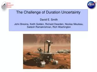
The Challenge of Duration Uncertainty. David E. Smith John Bresina, Keith Golden, Richard Dearden, Nicolas Meuleau, Sailesh Ramakrishnan, Rich Washington. Outline. The Problem objectives (goals) actions Approaches (neo-) classical MDP heuristic augmentation. Operational Characteristics.

E N D
The Challenge of Duration Uncertainty David E. Smith John Bresina, Keith Golden, Richard Dearden, Nicolas Meuleau, Sailesh Ramakrishnan, Rich Washington
Outline • The Problem • objectives (goals) • actions • Approaches • (neo-) classical • MDP • heuristic augmentation
Operational Characteristics • Brain dead • radiation • power • Safety • no risky operations • Communication • twice/day
Operational Characteristics • Brain dead • radiation • power • Safety • no risky operations • Communication • twice/day 3. Uplink 1. Plan on the ground Compress long …………… Visual servo (.2, -.15) Dig(5) Drive(-1) NIR Drive(2) Warmup NIR 2. Extensive checking/simulation
The Planning Problem • Initial conditions • start time • pose • power available • … • Possible science objectives • images • samples Compress Visual servo (.2, -.15) Dig(5) Drive(-1) NIR Drive(2) …………… Warmup NIR Maximize Scientific Return
The Objectives • Initial conditions • start time • pose • power available • … • Possible science objectives • images • samples • Decision Theoretic: • objectives are valued • choose Compress v=100 v=30 Visual servo (.2, -.15) Dig(5) Drive(-1) NIR Drive(2) …………… Warmup NIR Maximize Scientific Return
The Real Problem E > .1 Ah = .05 Ah = .02 Ah E > .6 Ah = .2 Ah = .2 Ah E > 3 Ah = 2 Ah = .5 Ah E > 7 Ah = 5 Ah = 2.5 Ah V = 10 Compress t [10:00, 14:00] = 600s = 60s = 1000s = 500s = 60s = 1s = 40s = 20s …………… Visual servo (.2, -.15) Dig(60) Drive (-1) NIR Drive (2) …………… V = 100 Warmup NIR = 400s = 20s E > 5 Ah = 3 Ah = .5 Ah
Uncertain Usage Uncertain resource usage E > .1 Ah = .05 Ah = .02 Ah E > .6 Ah = .2 Ah = .2 Ah E > 3 Ah = 2 Ah = .5 Ah E > 7 Ah = 5 Ah = 2.5 Ah V = 10 Compress t [10:00, 14:00] = 600s = 60s = 1000s = 500s = 60s = 1s Uncertain durations = 40s = 20s Visual servo (.2, -.15) Dig(60) Drive (-1) NIR Drive (2) …………… V = 100 Warmup NIR = 400s = 20s E > 5 Ah = 3 Ah = .5 Ah
Time & Resource Constraints Resource constraints E > .1 Ah = .05 Ah = .02 Ah E > .6 Ah = .2 Ah = .2 Ah E > 3 Ah = 2 Ah = .5 Ah E > 7 Ah = 5 Ah = 2.5 Ah V = 10 Compress Time constraints t [10:00, 14:00] = 600s = 60s = 1000s = 500s = 60s = 1s = 40s = 20s Visual servo (.2, -.15) Dig(60) Drive (-1) NIR Drive (2) …………… V = 100 Warmup NIR = 400s = 20s E > 5 Ah = 3 Ah = .5 Ah
E > .02 Ah = .01 Ah = 0 Ah E > 10 Ah = 5 Ah = 2.5 Ah E > .1 Ah = .05 Ah = .02 Ah E > .6 Ah = .2 Ah = .2 Ah t [9:00, 14:30] = 5s = 1s HiRes V = 10 t [10:00, 14:00] = 600s = 60s E > 3 Ah = 2 Ah = .5 Ah = 1000s = 500s = 60s = 1s = 40s = 20s Visual servo (.2, -.15) Dig(60) Drive (-2) NIR V = 100 t [9:00, 16:00] = 5s = 1s t [10:00, 13:50] = 600s = 60s = 120s = 20s Lo res Rock finder NIR V = 50 V = 5 E > .02 Ah = .01 Ah = 0 Ah E > .12 Ah = .1 Ah = .01 Ah E > 3 Ah = 2 Ah = .5 Ah How hard is it?
Utility 20 13:20 15 13:40 10 14:00 Power 5 Start time 14:20 14:40 How hard is it?
E > .02 Ah = .01 Ah = 0 Ah E > 10 Ah = 5 Ah = 2.5 Ah E > .1 Ah = .05 Ah = .02 Ah E > .6 Ah = .2 Ah = .2 Ah t [9:00, 14:30] = 5s = 1s HiRes V = 10 Utility t [10:00, 14:00] = 600s = 60s E > 3 Ah = 2 Ah = .5 Ah = 1000s = 500s = 60s = 1s = 40s = 20s Visual servo (.2, -.15) Dig(60) Drive (-2) NIR V = 100 20 t [9:00, 16:00] = 5s = 1s t [10:00, 13:50] = 600s = 60s 13:20 15 = 120s = 20s 13:40 10 Lo res Rock finder NIR V = 50 V = 5 14:00 E > .02 Ah = .01 Ah = 0 Ah E > .12 Ah = .1 Ah = .01 Ah E > 3 Ah = 2 Ah = .5 Ah 5 Power 14:20 Start time 14:40 Whazzzzup?
Visual servo (.2, -.15) Lo res Rock finder NIR Warmup NIR ∆t = ∆p = The Culprits Continuous time (& resources) Continuous outcomes Time (& resource) constraints Concurrency Power Storage Time t [10:00, 14:00] E > 2 Ah NIR
Visual servo (.2, -.15) Lo res Rock finder NIR Warmup NIR ∆t = ∆p = The Culprits Continuous time (& resources) Continuous outcomes Time (& resource) constraints Concurrency Power Storage Time t [10:00, 14:00] E > 2 Ah NIR Goal choices Optimization Simplicity constraints
Outline • The Problem • objectives (goals) • actions • Approaches • (neo-) classical • MDP • Heuristic augmentation
Disjunction Probability CGP CMBP C-PLAN Fragplan Non Observable Buridan UDTPOP p SENSp Cassandra PUCCINI SGP QBF-Plan GPT MBP C-Buridan DTPOP C-MAXPLAN ZANDER Mahinur ¬p Partially Observable Goal selection & optimization STRIPS model of action no concurrency no time no resources Discrete action outcomes JIC Plinth Weaver PGP Fully Observable WARPLAN-C CNLP Classical Planning under Uncertainty Problems
p ¬p STRIPS model of action no concurrency no time no resources Discrete action outcomes MDP’s & POMDPS Advantages Disjunction Probability Goal selection &optimization CGP CMBP C-PLAN Fragplan Non Observable Buridan UDTPOP SENSp Cassandra PUCCINI SGP QBF-Plan GPT MBP C-Buridan DTPOP C-MAXPLAN ZANDER Mahinur POMDPs Partially Observable Problems JIC Plinth Weaver PGP MDPs Fully Observable WARPLAN-C CNLP
Outline • The Problem • objectives (goals) • actions • Approaches • (neo-) classical • MDP • Heuristic • Conservative planning • Augmentation
Utility 20 13:20 15 13:40 10 14:00 5 Power 14:20 Start time 14:40 Conservative Planning Assume Dt= + t [9:00, 14:30] = 5s = 1s t=13:40 t=14:05 t=14:06 t=14:07 1500s HiRes V = 10 t [10:00, 14:00] = 600s = 60s = 1000s = 500s = 60s = 1s = 40s = 20s Visual servo (.2, -.15) Dig(60) Drive (-2) NIR V = 100 t [9:00, 16:00] = 5s = 1s t [10:00, 13:50] = 600s = 60s = 120s = 20s Lo res Rock finder NIR V = 50 V = 5
Heuristic Augmentation Plan based on expectations Analyze utility of result Augment add a branch
Just in Case (JIC) Scheduling 1. Seed schedule 2. Identify most likely failure 3. Generate a contingency branch 4. Integrate the branch .1 .4 .2 • Advantages: • Tractable • Simple plans • Anytime
Utility 20 13:20 15 13:40 10 14:00 5 Power 14:20 Start time 14:40 The Seed Assume Dt= t=13:35 t=13:52 t=13:53 t=13:54 t [10:00, 14:00] = 600s = 60s = 1000s = 500s = 60s = 1s = 40s = 20s Visual servo (.2, -.15) Dig(60) Drive (-2) NIR V = 100 V = 50
Utility 20 13:20 15 13:40 10 14:00 5 Power 14:20 Start time 14:40 Failure Point t=13:35 t=13:52 t=13:53 t=13:54 t [10:00, 14:00] = 600s = 60s = 1000s = 500s = 60s = 1s = 40s = 20s Visual servo (.2, -.15) Dig(60) Drive (-2) NIR V = 100
Utility 20 13:20 15 13:40 10 14:00 5 Power 14:20 Start time 14:40 Failure Point Assume Dt= t [9:00, 14:30] = 5s = 1s HiRes V = 10 t=13:35 t=13:52 t=13:53 t=13:54 t [10:00, 14:00] = 600s = 60s = 1000s = 500s = 60s = 1s = 40s = 20s Visual servo (.2, -.15) Dig(60) Drive (-2) NIR V = 100
Where the Branch *Should* Go t [9:00, 14:30] = 5s = 1s HiRes V = 10 1500s t=13:40 t=14:05 t=14:10 t=14:12 t [10:00, 14:00] = 600s = 60s = 1000s = 500s = 300s = 5s = 120s = 60s Visual servo (.2, -.15) Dig(60) Drive (-2) NIR V = 100 t [9:00, 16:00] = 5s = 1s t [10:00, 14:30] = 600s = 60s = 120s = 20s Lo res Rock finder LIB V = 50 V = 5 Warmup LIB = 1200s = 20s
Why? t [9:00, 14:30] = 5s = 1s HiRes V = 10 1500s t=13:40 t=14:05 t=14:10 t=14:12 t [10:00, 14:00] = 600s = 60s = 1000s = 500s = 300s = 5s = 120s = 60s Intermediate steps No inherent value Low impact on P Value of alternatives higher Visual servo (.2, -.15) Dig(60) Drive (-2) NIR V = 100 t [9:00, 16:00] = 5s = 1s t [10:00, 14:30] = 600s = 60s = 120s = 20s Lo res Rock finder LIB V = 50 V = 5 Warmup LIB = 1200s = 20s
Just in Case (JIC) Planning 1. Seed plan 2. Identify best branch point 3. Generate a contingency branch 4. Integrate the branch ? ? ?
Evaluating Branch Points Probability distributions for time & resources Utility of current plan as a function of time & resources Expected utility of a branch as a function of time & resources Branch condition Utility gain t=13:35 t [10:00, 14:00] = 600s = 60s = 1000s = 500s = 60s = 1s = 40s = 20s Visual servo (.2, -.15) Dig(60) Drive (-2) NIR V = 100
Estimating Branch Utility Probability distributions for time & resources Utility of current plan as a function of time & resources Expected utility of a branch as a function of time & resources Build PlanGraph Back-propagate utility distributions t=13:35 t [10:00, 14:00] = 600s = 60s = 1000s = 500s = 60s = 1s = 40s = 20s Visual servo (.2, -.15) Dig(60) Drive (-2) NIR V = 100
Visual servo (.2, -.15) Lo res Rock finder NIR Warmup NIR ∆t = ∆p = Final Points Continuous time (& resources) Continuous outcomes Time (& resource) constraints Concurrency Nasty combination! Power Storage Time • Existing approaches • painfully inadequate • Pervasive to • observation planning t [10:00, 14:00] E > 2 Ah World has round dice NIR