Machine Learning and Data Mining Regression Problem

1. + Machine Learning and Data MiningRegression Problem (adapted from) Prof. Alexander Ihler TexPoint fonts used in EMF. Read the TexPoint manual before you delete this box.: AAA

2. Overview • Regression Problem Definition and define parameters ϴ. • Prediction using ϴ as parameters • Measure the error • Finding good parameters ϴ (direct minimization problem) • Non-Linear regression problem (c) Alexander Ihler

3. Example of Regression • Vehicle price estimation problem • Features x: Fuel type, The number of doors, Engine size • Targets y: Price of vehicle • Training Data: (fit the model) • Testing Data: (evaluate the model)

4. Example of Regression • Vehicle price estimation problem • ϴ = [-300, -200 , 700 , 130] • Ex #1 = -300 + -200 *1 + 4*700 + 70*130 = 11400 • Ex #2 = -300 + -200 *1 + 2*700 + 120*130 = 16500 • Ex #3 = -300 + -200 *2 + 2*700 + 310*130 = 41000 • Mean Absolute Training Error = 1/3 *(400 + 500 + 0) = 300 • Test = -300 + -200 *2 + 4*700 + 150*130 = 21600 • Mean Absolute Testing Error = 1/1 *(600) = 600

5. Supervised learning • Notation • Features x (input variables) • Targets y (output variables) • Predictions ŷ • Parameters q • Error = Distance between y and ŷ Learning algorithm Change θ Improve performance Program (“Learner”) Characterized by some “parameters”θ Procedure (using θ) that outputs a prediction Training data (examples) Features Feedback / Target values Evaluation of the model (measure error)

6. Overview • Regression Problem Definition and parameters. • Prediction using ϴ as parameters • Measure the error • Finding good parameters ϴ (direct minimization problem) • Non-Linear regression problem (c) Alexander Ihler

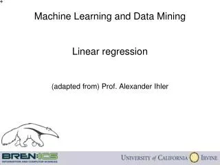
7. Linear regression “Predictor”: Evaluate line: ӯ = ϴ0 +ϴ1 * X1 return ӯ ӯ = Predicted target value (Black line) • Define form of function f(x) explicitly • Find a good f(x) within that family New instance with X1=8 Predicted value =17 40 Y = 5 + 1.5*X1 Target y 20 0 0 10 20 Feature X1 (c) Alexander Ihler

8. 26 26 24 24 y 22 22 20 20 30 30 40 40 20 20 30 30 x1 20 20 x2 10 10 10 10 0 0 0 0 More dimensions? y x1 x2 (c) Alexander Ihler

9. Notation Ӯ is a plane in n+1 dimension space Define “feature” x0 = 1 (constant) Then n = the number of features in dataset (c) Alexander Ihler

10. Overview • Regression Problem Definition and parameters. • Prediction using ϴ as parameters • Measure the error • Finding good parameters ϴ (direct minimization problem) • Non-Linear regression problem (c) Alexander Ihler

11. Supervised learning • Notation • Features x (input variables) • Targets y (output variables) • Predictions ŷ • Parameters q • Error = Distance between y and ŷ Learning algorithm Change θ Improve performance Program (“Learner”) Characterized by some “parameters”θ Procedure (using θ) that outputs a prediction Training data (examples) Features Feedback / Target values Evaluation of the model (measure error)

12. Red points = Real target values Black line = ӯ (predicted value) ӯ = ϴ0 +ϴ1 * X Blue lines = Error (Difference between real value y and predicted value ӯ) Measuring error Error or “residual” Observation Prediction 0 0 20 (c) Alexander Ihler

13. Mean Squared Error • How can we quantify the error? • Y= Real target value in dataset, • ӯ = Predicted target value by ϴ*X • Training Error: m= the number of training instances, • Testing Error: Using a partition of Training error to check predicted values. m= the number of testing instances, m=number of instance of data (c) Alexander Ihler

14. MSE cost function • Rewrite using matrix form X = input variables in dataset y= output variable in dataset m=number of instance of data n = the number of features, (Matlab) >> e = y’ – th*X’; J = e*e’/m; (c) Alexander Ihler

15. Visualizing the error function J is error function. The plane is the value of J, not the plane fitted to output values. Dimensions are ϴ0 and ϴ1instead of X1 and X2 Output is J instead of y as target value J(θ) θ0 θ1 Representation of J in 2D space. Inner red circles has less value of J Outer red circles has higher value of J θ1 (c) Alexander Ihler θ0 θ 0

16. Overview • Regression Problem Definition and parameters. • Prediction using ϴ as parameters • Measure the error • Finding good parameters ϴ (direct minimization problem) • Non-Linear regression problem (c) Alexander Ihler

17. Supervised learning • Notation • Features x • Targets y • Predictions ŷ • Parameters q Learning algorithm Change θ Improve performance Program (“Learner”) Characterized by some “parameters”θ Procedure (using θ) that outputs a prediction Training data (examples) Features Feedback / Target values Evaluation of the model (measure error)

18. Finding good parameters • Want to find parameters which minimize our error… • Think of a cost “surface”: error residual for that θ… (c) Alexander Ihler

19. MSE Minimum (m <= n+1) m=number of instance of data n = the number of features, • Consider a simple problem • One feature, two data points • Two unknowns and two equations: n +1=1+1 = 2 m=2 • Can solve this system directly: Theta gives a line or plane that exactly fit to all target values. (c) Alexander Ihler

20. SSE Minimum (m > n+1) • Reordering, we have • Most of the time, m > n • There may be no linear function that hits all the data exactly • Minimum of a function has gradient equal to zero (gradient is a horizontal line.) n +1=1+1 = 2 m=3 Just need to know how to compute parameters. (c) Alexander Ihler

21. 18 16 14 162 cost for this one datum Heavy penalty for large errors Distract line from other points. 12 10 8 6 4 2 0 0 2 4 6 8 10 12 14 16 18 20 Effects of Mean Square Error choice outlier data: An outlier is an observation that lies an abnormal distance from other value. (c) Alexander Ihler

22. Absolute error MSE, original data 18 Abs error, original data 16 Abs error, outlier data 14 12 10 8 6 4 2 0 0 2 4 6 8 10 12 14 16 18 20 (c) Alexander Ihler

23. Something else entirely… Error functions for regression (Mean Square Error) (Mean Absolute Error) (???) “Arbitrary”Error functions can’t be solved in closed form… So as alternative way, use gradient descent (c) Alexander Ihler

24. Overview • Regression Problem Definition and parameters. • Prediction using ϴ as parameters • Measure the error • Finding good parameters ϴ (direct minimization problem) • Non-Linear regression problem (c) Alexander Ihler

25. Nonlinear functions • Single feature x, predict target y: • Sometimes useful to think of “feature transform” • Convert a non-linear function to linear function and then solve it. Add features: Linear regression in new features (c) Alexander Ihler

26. Higher-order polynomials Y = ϴ0 • Are more features better? • “Nested” hypotheses • 2nd order more general than 1st, • 3rd order ““ than 2nd, … • Fits the observed data better Y = ϴ0+ ϴ1 * X Y = ϴ0+ ϴ1 * X + ϴ2*X2 + ϴ3*X3 18nd order 3rd order 1st order

27. Test data • After training the model • Go out and get more data from the world • New observations (x,y) • How well does our model perform? Training data New, “test” data (c) Alexander Ihler

28. Plot MSE as a function of model complexity Polynomial order Decreases More complex function fits training data better What about new data? 30 Training data 25 New, “test” data 20 15 • 0th to 2storder • Error decreases • Underfitting • Higher order • Error increases • Overfitting 10 5 0 0 1 2 3 4 5 6 7 8 9 10 Training versus test error Under fitting Overfitting Mean squared error Polynomial order (c) Alexander Ihler

29. Summary • Regression Problem Definition • Vehicle Price estimation • Prediction using ϴ: • Measure the error: difference between y and ŷ • e.g. Absolute error, MSE • direct minimization problem • Two cases m<=n+1 and m > n+1 • Non-Linear regression problem • Finding best nth order polynomial function for each problem (not overfitting and not under fitting)