Lossless Compression Algorithms: An Overview
Explore the basics of lossless compression through run-length coding, variable-length coding, Huffman coding, and more in information theory. Learn about entropy, coding schemes, and algorithms used for efficient data compression.

Lossless Compression Algorithms: An Overview
E N D
Presentation Transcript
Chapter 7Lossless Compression Algorithms 7.1 Introduction 7.2 Basics of Information Theory 7.3 Run-Length Coding 7.4 Variable-Length Coding (VLC) 7.5 Dictionary-based Coding 7.6 Arithmetic Coding 7.7 Lossless Image Compression Li & Drew
7.1 Introduction • • Compression: the process of coding that will effectively reduce the total number of bits needed to represent certain information. • Fig. 7.1: A General Data Compression Scheme. Li & Drew
Introduction (cont’d) • • If the compression and decompression processes induce no information loss, then the compression scheme is lossless; otherwise, it is lossy. • • Compression ratio: • (7.1) • B0 – number of bits before compression • B1 – number of bits after compression Li & Drew
7.2 Basics of Information Theory • • The entropyη of an information source with alphabet S = {s1, s2, . . . , sn} is: • (7.2) • (7.3) • pi – probability that symbol si will occur in S. • – indicates the amount of information ( self-information as defined by Shannon) contained in si, which corresponds to the number of bits needed to encode si. Li & Drew
Distribution of Gray-Level Intensities • Fig. 7.2 Histograms for Two Gray-level Images. • • Fig. 7.2(a) shows the histogram of an image with uniform distribution of gray-level intensities, i.e., ∀i pi= 1/256. Hence, the entropy of this image is: • log2256 = 8 (7.4) • • Fig. 7.2(b) shows the histogram of an image with two possible values. Its entropy is 0.92. Li & Drew
Entropy and Code Length • • As can be seen in Eq. (7.3): the entropy η is a weighted-sum of terms ; hence it represents the average amount of information contained per symbol in the source S. • • The entropy η specifies the lower bound for the average number of bits to code each symbol in S, i.e., • (7.5) • - the average length (measured in bits) of the codewords produced by the encoder. Li & Drew
7.3 Run-Length Coding • • Memoryless Source: an information source that is independently distributed. Namely, the value of the current symbol does not depend on the values of the previously appeared symbols. • • Instead of assuming memoryless source, Run-Length Coding (RLC) exploits memory present in the information source. • • Rationale for RLC: if the information source has the property that symbols tend to form continuous groups, then such symbol and the length of the group can be coded. Li & Drew
7.4 Variable-Length Coding (VLC) • Shannon-Fano Algorithm — a top-down approach • 1. Sort the symbols according to the frequency count of their occurrences. • 2. Recursively divide the symbols into two parts, each with approximately the same number of counts, until all parts contain only one symbol. • An Example: coding of “HELLO” • Frequency count of the symbols in ”HELLO”. Li & Drew
Table 7.1: Result of Performing Shannon-Fano on HELLO Li & Drew
Fig. 7.4 Another coding tree for HELLO by Shannon-Fano. Li & Drew
Table 7.2: Another Result of Performing Shannon-Fano • on HELLO (see Fig. 7.4) Li & Drew
Huffman Coding • ALGORITHM 7.1 Huffman Coding Algorithm— a bottom-up approach • 1. Initialization: Put all symbols on a list sorted according to their frequency counts. • 2. Repeat until the list has only one symbol left: • (1) From the list pick two symbols with the lowest frequency counts. Form a Huffman subtree that has these two symbols as child nodes and create a parent node. • (2) Assign the sum of the children’s frequency counts to the parent and insert it into the list such that the order is maintained. • (3) Delete the children from the list. • 3. Assign a codeword for each leaf based on the path from the root. Li & Drew
Fig. 7.5: Coding Tree for “HELLO” using the Huffman Algorithm. Li & Drew
Huffman Coding (cont’d) • In Fig. 7.5, new symbols P1, P2, P3 are created to refer to the parent nodes in the Huffman coding tree. The contents in the list are illustrated below: • After initialization: L H E O • After iteration (a): L P1 H • After iteration (b): L P2 • After iteration (c): P3 Li & Drew
Properties of Huffman Coding • 1. Unique Prefix Property: No Huffman code is a prefix of any other Huffman code - precludes any ambiguity in decoding. • 2. Optimality: minimum redundancy code - proved optimal for a given data model (i.e., a given, accurate, probability distribution): • • The two least frequent symbols will have the same length for their Huffman codes, differing only at the last bit. • • Symbols that occur more frequently will have shorter Huffman codes than symbols that occur less frequently. • * Huffman Coding has been adopted in fax machines, JPEG, and MPEG. Li & Drew
7.5 Dictionary-based Coding • • Lempel-Ziv-Welch (LZW) algorithm uses fixed-length codewords to represent variable-length strings of symbols/characters that commonly occur together, e.g., words in English text. • • the LZW encoder and decoder build up the same dictionary dynamically while receiving the data. • • LZW places longer and longer repeated entries into a dictionary, and then emits the code for an element, rather than the string itself, if the element has already been placed in the dictionary. • • UNIX compress, GIF images, and V.42bis for modems. Li & Drew
7.6 Arithmetic Coding • • Arithmetic coding is a more modern coding method that usually out-performs Huffman coding. • • Huffman coding assigns each symbol a codeword which has an integral bit length. Arithmetic coding can treat the whole message as one unit. • • A message is represented by a half-open interval [a, b) where a and b are real numbers between 0 and 1. Initially, the interval is [0, 1). When the message becomes longer, the length of the interval shortens and the number of bits needed to represent the interval increases. Li & Drew
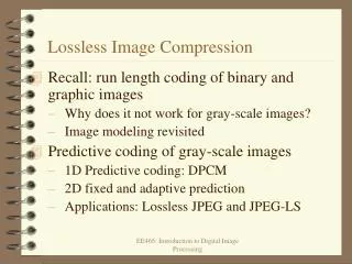
7.7 Lossless Image Compression • • Approaches of Differential Coding of Images: • – Given an original image I(x, y), using a simple difference operator we can define a difference image d(x, y) as follows: • d(x, y) = I(x, y) − I(x − 1, y) (7.9) • or use the discrete version of the 2-D Laplacian operator to define a difference image d(x, y) as • d(x, y) = 4 I(x, y) − I(x, y − 1) − I(x, y +1) − I(x+1, y) − I(x − 1, y) • (7.10) • • Due to spatial redundancy existed in normal images I, the difference image d will have a narrower histogram and hence a smaller entropy, as shown in Fig. 7.9. Li & Drew
Fig. 7.9: Distributions for Original versus Derivative Images. (a,b): Original gray-level image and its partial derivative image; (c,d): Histograms for original and derivative images. • (This figure uses a commonly employed image called “Barb”.) Li & Drew
Lossless JPEG • • Lossless JPEG: A special case of the JPEG image compression. • • The Predictive method • 1. Forming a differential prediction: A predictor combines the values of up to three neighboring pixels as the predicted value for the current pixel, indicated by ‘X’ in Fig. 7.10. The predictor can use any one of the seven schemes listed in Table 7.6. • 2. Encoding: The encoder compares the prediction with the actual pixel value at the position ‘X’ and encodes the difference using one of the lossless compression techniques we have discussed, e.g., the Huffman coding scheme. Li & Drew
Fig. 7.10: Neighboring Pixels for Predictors in Lossless JPEG. • • Note: Any of A, B, or C has already been decoded before it is used in the predictor, on the decoder side of an encode-decode cycle. Li & Drew
Table 7.6: Predictors for Lossless JPEG Li & Drew
Table 7.7: Comparison with other lossless compression programs See this: http://www.cs.sfu.ca/mmbook/furtherv2/node7.html Li & Drew