Recall Taylor’s Theorem from single variable calculus:
110 likes | 135 Vues
Recall Taylor’s Theorem from single variable calculus:. If y = f ( x ) is a function with continuous derivatives up to order k + 1 (that is, f is differentiable up to order k + 1) at x 0 , then. f ( x 0 ) ——— h 2 +... 2!. f ( k ) ( x 0 ) + ——— h k + k !.

Recall Taylor’s Theorem from single variable calculus:
E N D
Presentation Transcript
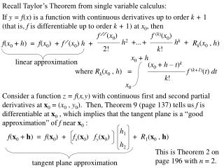
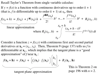
Recall Taylor’s Theorem from single variable calculus: If y = f(x) is a function with continuous derivatives up to order k + 1 (that is, f is differentiable up to order k + 1) at x0, then f (x0) ——— h2 +... 2! f (k)(x0) + ——— hk + k! f(x0 + h) = f(x0) + f (x0) h + Rk(x0 , h) x0 + h (x0 + h – t)k ————— f (k+1)(t) dt k! x0 linear approximation where Rk(x0 , h) = Consider a function z = f(x,y) with continuous first and second partial derivatives at x0 = (x0 , y0). Then, Theorem 9 (page 137) tells us f is differentiable at x0 , which implies that the tangent plane is a “good approximation” of f near x0 : h1 h2 f(x0 + h) = f(x0) + fx(x0) fy(x0) + R1(x0 , h) This is Theorem 2 on page 196 with n = 2. tangent plane approximation
Consider a function z = f(x,y) with continuous first, second, and third partial derivatives at x0 = (x0 , y0). Then, by defining g(t) = f(x0 + th) and applying the second order Taylor polynomial from single variable calculus (by using the chain rule), we get Theorem 3 on page 196 with n = 2 : h1 h2 This matrix of second derivatives is called the Hessian matrix. f(x0 + h) = f(x0) + fx(x0) fy(x0) linear approximation fxx(x0) fyx(x0) fxy(x0) fyy(x0) h1 h2 1 — 2 + h1h2 + R2(x0 , h) quadratic approximation
Consider a function z = f(x,y) with continuous first, second, and third partial derivatives at x0 = (x0 , y0). Then, by defining g(t) = f(x0 + th) and applying the second order Taylor polynomial from single variable calculus (by using the chain rule), we get Theorem 3 on page 196 with n = 2 : fx(x0) h1 + fy(x0) h2 h1 h2 f(x0 + h) = f(x0) + fx(x0) fy(x0) fxx(x0) fyx(x0) fxy(x0) fyy(x0) h1 h2 1 — 2 + h1h2 1 — 2 1 — 2 fxx(x0) h12 + fxy(x0) h1h2 + fyy(x0) h22 + R2(x0 , h)
Find the second-order Taylor polynomial for f(x,y) = ex cos y at the point x0 = (x0 , y0) = (0,0) . f(0,0) = fx = fx(0,0) = fy = fy(0,0) = fxx = fxx(0,0) = fyy = fyy(0,0) = fxy = fxy(0,0) = 1 ex cos y 1 – ex sin y 0 ex cos y 1 – ex cos y – 1 – ex sin y 0 x– x0 y– y0 f(x0 + h) = f(h) = f(h1 , h2) = 1 —(–1)(h2)2 2 1 — (1)(h1)2 + 2 (1)(h1) + (0)(h2) + 1 + (0)(h1)(h2) + + R2(0 , h) x x2 y2 1 1 = 1 + h1 + — h12 – — h22 + R2(0 , h) 2 2
Find the second-order Taylor polynomial for f(x,y) = sin(x + 2y) at the point x0 = (x0 , y0) = (0,0) . f(0,0) = fx = fx(0,0) = fy = fy(0,0) = fxx = fxx(0,0) = fyy = fyy(0,0) = fxy = fxy(0,0) = 0 cos(x + 2y) 1 2 cos(x + 2y) 2 – sin(x + 2y) 0 – 4sin(x + 2y) 0 – 2sin(x + 2y) 0 f(x0 + h) = f(h) = f(h1 , h2) = 1 —(0)(h2)2 2 1 —(0)(h1)2 + 2 (1)(h1) + (2)(h2) + 0 + (0)(h1)(h2) + + R2(0 , h) = h1 + 2h2 + R2(0 , h) Note that the first-order and second-order Taylor polynomials are identical!
Find the first-order and second-order Taylor approximations to f(x,y) = sin(xy) at the point x0 = (x0 , y0) = (1 , /2) . f(1 , /2) = fx = fx(1 , /2) = fy = fy(1 , /2) = fxx = fxx(1 , /2) = fyy = fyy(1 , /2) = fxy = fxy(1 , /2) = 1 y cos(xy) 0 x cos(xy) 0 – y2sin(xy) –2/4 – x2sin(xy) – 1 cos(xy) – xy sin(xy) –/2 f(x0 + h) = f(1 + h1 , /2 + h2) = f(x,y) = (0)(x – 1) + (0)(y – /2) + 1 + 1 —(–1)(y – /2)2 2 1 —(–2/4)(x – 1)2 + 2 (–/2)(x – 1)(y – /2) + + R2((1 , /2) , h) 1 The first-order (linear) approximation is sin(xy) The second-order (quadratic) approximation is sin(xy)
Find the first-order and second-order Taylor approximations to f(x,y) = sin(xy) at the point x0 = (x0 , y0) = (1 , /2) . f(x0 + h) = f(1 + h1 , /2 + h2) = f(x,y) = (0)(x – 1) + (0)(y – /2) + 1 + 1 —(–1)(y – /2)2 2 1 —(–2/4)(x – 1)2 + 2 (–/2)(x – 1)(y – /2) + + R2(0 , h) 1 The first-order (linear) approximation is sin(xy) The second-order (quadratic) approximation is sin(xy) 2 1 1 – —(x – 1)2 – —(x – 1)(y – /2) – —(y – /2)2 8 2 2
Find the linear and quadratic Taylor approximations to the expression (3.98 – 1)2 / (5.97 – 3)2 . Compare these approximations with the exact value. We shall find the linear and quadratic Taylor approximations to f(x,y) = at the point x0 = (x0 , y0) = ( , ) . (x– 1)2 / (y – 3)2 4 6 f(4,6) = fx = fx(4,6) = fy = fy(4,6) = fxx = fxx(4,6) = fyy = fyy(4,6) = fxy = fxy(4,6) = 2(x– 1) / (y – 3)2 2/3 1 –2(x–1)2 / (y –3)3 – 2/3 2 / (y – 3)2 2/9 6(x– 1)2 / (y – 3)4 2/3 –4(x– 1) / (y – 3)3 – 4/9 f(x0 + h) = f(4 + h1 , 6 + h2) = f(x,y) = (2/3)(x – 4) + (–2/3)(y – 6) + 1 + 1 —(2/9)(x – 4)2 + 2 1 —(2/3)(y – 6)2 2 (–4/9)(x – 4)(y – 6) + + R2((4,6) , h)
Find the linear and quadratic Taylor approximations to the expression (3.98 – 1)2 / (5.97 – 3)2 . Compare these approximations with the exact value. We shall find the linear and quadratic Taylor approximations to f(x,y) = at the point x0 = (x0 , y0) = ( , ) . (x– 1)2 / (y – 3)2 4 6 f(x0 + h) = f(4 + h1 , 6 + h2) = f(x,y) = (2/3)(x – 4) + (–2/3)(y – 6) + 1 + 1 —(2/3)(y – 6)2 2 1 —(2/9)(x – 4)2 + 2 (–4/9)(x – 4)(y – 6) + + R2((4,6) , h) The linear approximation of (3.98 – 1)2 / (5.97 – 3)2 is 1 + (2/3)(–0.02) + (–2/3)(–0.03) = 1.00666 The quadratic approximation of (3.98 – 1)2 / (5.97 – 3)2 is 1 + (2/3)(–0.02) + (–2/3)(–0.03) + (1/9)(–0.02)2 + (–4/9)(–0.02)(–0.03) + (1/3)(–0.03)2 = 1.00674 The “exact” value is 1.00675.
The Second Order Taylor Formula is really just the terms in a power series expansion up to degree two. If we know the power series expansion, then we can extract the terms that would be in the Second Order (or any order!) Taylor Formula. For example, we know that for –1 < r < 1, 1 + r + r2 + r3 + r4 +... = 1 —— 1 – r
Consider the function 1 1 f(x,y) = ———— = ———— 1 – x – y2 1 – (x + y2) We can obtain the linear and quadratic approximations (or any other order approximations!) from the fact that 1 f(x,y) = ———— = 1 – (x + y2) for –1 < x + y2 < 1 1 + (x + y2) + (x + y2)2 + (x + y2)3 + … . The first order Taylor formula is f(x,y) 1 + x The second order Taylor formula is f(x,y) 1 + x + x2 + y2 The third order Taylor formula is f(x,y) 1 + x + x2 + x3 + y2 + 2xy2