Matlab Tutorial. Session 2. SIFT
Matlab Tutorial. Session 2. SIFT. Gonzalo Vaca-Castano. Sift purpose. Find and describe interest points invariants to: Scale Rotation Illumination Viewpoint. Do it Yourself. Constructing a scale space LoG Approximation Finding keypoints

Matlab Tutorial. Session 2. SIFT
E N D
Presentation Transcript
Matlab Tutorial.Session 2.SIFT Gonzalo Vaca-Castano
Sift purpose • Find and describe interest points invariants to: • Scale • Rotation • Illumination • Viewpoint
Do it Yourself • Constructing a scale space • LoGApproximation • Finding keypoints • Get rid of bad key points (A technique similar to the Harris Corner Detector) • Assigning an orientation to the keypoints • Generate SIFT features *http://www.aishack.in/2010/05/sift-scale-invariant-feature-transform/2/
Construction of a scale space SIFT takes scale spaces to the next level. You take the original image, and generate progressively blurred out images. Then, you resize the original image to half size. And you generate blurred out images again. And you keep repeating. The creator of SIFT suggests that 4 octaves and 5 blur levels are ideal for the algorithm
Construction of a scale space (details) • The first octave • If the original image is doubled in size and antialiased a bit (by blurring it) then the algorithm produces more four times more keypoints. The more the keypoints, the better! • Blurring • Amount of Blurring
Matlab Implementation ! % %%% Create first interval of the first octave %%%%% init_image=impyramid(gauss_filter(image1,antialiassigma,4*antialiassigma),'expand'); gaussians(1)={gauss_filter(init_image,sigmavalue,4*sigmavalue)}; % %%% Generates all the blurred out images for each octave %%%% % %%% and the DoG images %%%% for i=1:num_octaves sigma=sigmavalue; %reset the sigma value for j=1:(num_intervals+2) sigma=sigma*2^((j-1)/2); %Assign a sigma value acording to the scale previmage=cell2mat(gaussians(j,i)); %Obtain the previous image newimage=gauss_filter(previmage,sigma,4*sigma); %apply a new smoothing dog=previmage-newimage; %calculate the difference of gaussians %save the results gaussians(j+1,i)={newimage}; dogs(j,i)={dog}; end %Build the init image in the next level if(i<num_octaves) lowscale=cell2mat(gaussians(num_intervals+1,i)); upscale=impyramid(lowscale,'reduce'); gaussians(1,i+1)={upscale}; end end
Finding keypoints • a) Locate maxima/minima in DoG images
Matlab Implementation for i=1:num_octaves for j=2:(num_intervals+1) % Obtain the matrices where to look for the extrema level=cell2mat(dogs(j,i)); up=cell2mat(dogs(j+1,i)); down=cell2mat(dogs(j-1,i)); [sx,sy]=size(level); %look for a local maxima local_maxima=(level(2:sx-1,2:sy-1)>level(1:sx-2,1:sy-2)) & ( level(2:sx-1,2:sy-1) > level(1:sx-2,2:sy-1) ) & (level(2:sx-1,2:sy-1)>level(1:sx-2,3:sy)) & (level(2:sx-1,2:sy-1)>level(2:sx-1,1:sy-2)) & (level(2:sx-1,2:sy-1)>level(2:sx-1,3:sy)) & (level(2:sx-1,2:sy-1)>level(3:sx,1:sy-2)) & (level(2:sx-1,2:sy-1)>level(3:sx,2:sy-1)) & (level(2:sx-1,2:sy-1)>level(3:sx,3:sy)) ; local_maxima=local_maxima & (level(2:sx-1,2:sy-1)>up(1:sx-2,1:sy-2)) & ( level(2:sx-1,2:sy-1) > up(1:sx-2,2:sy-1) ) & (level(2:sx-1,2:sy-1)>up(1:sx-2,3:sy)) & (level(2:sx-1,2:sy-1)>up(2:sx-1,1:sy-2)) & (level(2:sx-1,2:sy-1)>up(2:sx-1,2:sy-1)) & (level(2:sx-1,2:sy-1)>up(2:sx-1,3:sy)) & (level(2:sx-1,2:sy-1)>up(3:sx,1:sy-2)) & (level(2:sx-1,2:sy-1)>up(3:sx,2:sy-1)) & (level(2:sx-1,2:sy-1)>up(3:sx,3:sy)) ; local_maxima=local_maxima & (level(2:sx-1,2:sy-1)>down(1:sx-2,1:sy-2)) & ( level(2:sx-1,2:sy-1) > down(1:sx-2,2:sy-1) ) & (level(2:sx-1,2:sy-1)>down(1:sx-2,3:sy)) & (level(2:sx-1,2:sy-1)>down(2:sx-1,1:sy-2)) & (level(2:sx-1,2:sy-1)>down(2:sx-1,2:sy-1)) & (level(2:sx-1,2:sy-1)>down(2:sx-1,3:sy)) & (level(2:sx-1,2:sy-1)>down(3:sx,1:sy-2)) & (level(2:sx-1,2:sy-1)>down(3:sx,2:sy-1)) & (level(2:sx-1,2:sy-1)>down(3:sx,3:sy)) ; %look for a local minima local_minima=(level(2:sx-1,2:sy-1)>level(1:sx-2,1:sy-2)) & ( level(2:sx-1,2:sy-1) > level(1:sx-2,2:sy-1) ) & (level(2:sx-1,2:sy-1)>level(1:sx-2,3:sy)) & (level(2:sx-1,2:sy-1)>level(2:sx-1,1:sy-2)) & (level(2:sx-1,2:sy-1)>level(2:sx-1,3:sy)) & (level(2:sx-1,2:sy-1)>level(3:sx,1:sy-2)) & (level(2:sx-1,2:sy-1)>level(3:sx,2:sy-1)) & (level(2:sx-1,2:sy-1)>level(3:sx,3:sy)) ; local_minima=local_minima & (level(2:sx-1,2:sy-1)>up(1:sx-2,1:sy-2)) & ( level(2:sx-1,2:sy-1) > up(1:sx-2,2:sy-1) ) & (level(2:sx-1,2:sy-1)>up(1:sx-2,3:sy)) & (level(2:sx-1,2:sy-1)>up(2:sx-1,1:sy-2)) & (level(2:sx-1,2:sy-1)>up(2:sx-1,2:sy-1)) & (level(2:sx-1,2:sy-1)>up(2:sx-1,3:sy)) & (level(2:sx-1,2:sy-1)>up(3:sx,1:sy-2)) & (level(2:sx-1,2:sy-1)>up(3:sx,2:sy-1)) & (level(2:sx-1,2:sy-1)>up(3:sx,3:sy)) ; local_minima=local_minima & (level(2:sx-1,2:sy-1)>down(1:sx-2,1:sy-2)) & ( level(2:sx-1,2:sy-1) > down(1:sx-2,2:sy-1) ) & (level(2:sx-1,2:sy-1)>down(1:sx-2,3:sy)) & (level(2:sx-1,2:sy-1)>down(2:sx-1,1:sy-2)) & (level(2:sx-1,2:sy-1)>down(2:sx-1,2:sy-1)) & (level(2:sx-1,2:sy-1)>down(2:sx-1,3:sy)) & (level(2:sx-1,2:sy-1)>down(3:sx,1:sy-2)) & (level(2:sx-1,2:sy-1)>down(3:sx,2:sy-1)) & (level(2:sx-1,2:sy-1)>down(3:sx,3:sy)) ; extrema=local_maxima | local_minima; end end
Finding keypoints • b) Find subpixel maxima/minima
Get rid of bad key points • Removing low contrast features If the magnitude of the intensity (i.e., without sign) at the current pixel in the DoG image (that is being checked for minima/maxima) is less than a certain value, it is rejected • Removing edges
Matlab Implementation %indices of the extrema points [x,y]=find(extrema); numtimes=size(find(extrema)); for k=1:numtimes x1=x(k); y1=y(k); if(abs(level(x1+1,y1+1))<contrast_threshold) %low contrast point are discarded extrema(x1,y1)=0; else %keep being extrema, check for edge rx=x1+1; ry=y1+1; fxx= level(rx-1,ry)+level(rx+1,ry)-2*level(rx,ry); % double derivate in x direction fyy= level(rx,ry-1)+level(rx,ry+1)-2*level(rx,ry); % double derivate in y direction fxy= level(rx-1,ry-1)+level(rx+1,ry+1)-level(rx-1,ry+1)-level(rx+1,ry-1); %derivate inx and y direction trace=fxx+fyy; deter=fxx*fyy-fxy*fxy; curvature=trace*trace/deter; curv_threshold= ((r_curvature+1)^2)/r_curvature; if(deter<0 || curvature>curv_threshold) %Reject edge points extrema(x1,y1)=0; end end end
Generate SIFT features • You take a 16×16 window of “in-between” pixels around the keypoint. You split that window into sixteen 4×4 windows. From each 4×4 window you generate a histogram of 8 bins. Each bin corresponding to 0-44 degrees, 45-89 degrees, etc. Gradient orientations from the 4×4 are put into these bins. This is done for all 4×4 blocks. Finally, you normalize the 128 values you get. • To solve a few problems, you subtract the keypoint’s orientation and also threshold the value of each element of the feature vector to 0.2 (and normalize again).
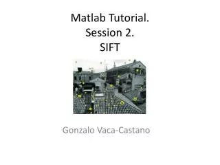
Testing the detector • i=imread('groceries_gray.jpg'); • sift(i,3,5,1.1)
Vl_feat • The VLFeat open source library implements popular computer vision algorithms including SIFT, MSER, k-means, hierarchical k-means, agglomerative information bottleneck, and quick shift. It is written in C for efficiency and compatibility, with interfaces in MATLAB for ease of use, and detailed documentation throughout. It supports Windows, Mac OS X, and Linux
Vl_feat • Download vl_feat from http://www.vlfeat.org/ • run('VLFEATROOT/toolbox/vl_setup') • Permanent setup • To permanently add VLFeat to your MATLAB environment, add this line to your startup.m file: • run('VLFEATROOT/toolbox/vl_setup')
Extracting frames and descriptors pfx = fullfile(vl_root,'data','a.jpg') ; I = imread(pfx) ; image(I) ; I = single(rgb2gray(I)) ; [f,d] = vl_sift(I) ; perm = randperm(size(f,2)) ; sel = perm(1:50) ; h1 = vl_plotframe(f(:,sel)) ; h2 = vl_plotframe(f(:,sel)) ; set(h1,'color','k','linewidth',3) ; set(h2,'color','y','linewidth',2) ; h3 = vl_plotsiftdescriptor(d(:,sel),f(:,sel)) ; set(h3,'color','g')
Basic Matching [fa, da] = vl_sift(Ia) ; [fb, db] = vl_sift(Ib) ; [matches, scores] = vl_ubcmatch(da, db) ;
Visualization • m1= fa (1:2,matches(1,:)); • m2=fb(1:2,matches(2,:)); • m2(1,:)= m2(1,:)+640*ones(1,size(m2,2)); • X=[m1(1,:);m2(1,:)]; • Y=[m1(2,:);m2(2,:)]; • imshow(c); • hold on; • line(X,Y) • vl_plotframe(aframe(:,matches(1,:))); • vl_plotframe(m2);
Custom frames • The MATLAB command vl_sift (and the command line utility) can bypass the detector and compute the descriptor on custom frames using the Frames option. • For instance, we can compute the descriptor of a SIFT frame centered at position (100,100), of scale 10 and orientation -pi/8 by • fc = [100;100;10;-pi/8] ; • [f,d] = vl_sift(I,'frames',fc) ; • fc = [100;100;10;0] ; • [f,d] = vl_sift(I,'frames',fc,'orientations') ;