Download
1 / 46
460 likes | 490 Vues
This chapter explores the concept of modeling in the study of system performance, including the types of models, performance metrics, and simulation techniques. It discusses the importance of abstraction and the different categories of models, such as physical, graphical, and mathematical models. The chapter also covers performance measures, such as average wait time and throughput, and the concepts of efficiency, reliability, and availability. Simulation models and their implementation are explained, along with how performance goals are set for internal subsystems.

E N D
Systems and Models • The concept of modeling in the study of the dynamic behavior of simple system is be able to calculating their performances. • System is the part of the real world under study, which composed of a set of entities interacting among themselves and with the environment. • A model is an abstract representation of a system. • The system behavior is dependent on the input data and actions from the environment.
Abstraction • The most important concept in analysis and design • It hide nonessential properties and behavior of the system so the model is used to describe, study, and/or design the system. • A high-level description of a collection of objects • Only the relevant properties and features of the objects are included.
System A system has: • Structure • Behavior The model of a system is simpler than the real system in its structure and behavior. But it should be equivalent to the system.
Using Models A user can: • Manipulate the model by supplying it with a set of inputs • Observe its behavior and/or measure its output when given some input/output. • Predict the behavior of the real system by analyzing the behavior of the model under the same circumstances.
Types of Model The most general categories of models are: • Physical models (scale models) is resemble the physical attributes of an actual object by scaling down the physical system. • Graphical models use graphical representations to display the behavior of a system. • Mathematical models is a set of Mathematical expression and logical relations to express the relationships among the entities of objects of the system. • Models are the most flexible ones and are the ones studied here.
Mathematical Models • Analytic, the solution is a set of expressions that define the behavior of the model. • Numeric, mathematical techniques are used to derive values for the model behavior within given intervals. • Deterministic and stochastic models are solved with numerical techniques.
Other Categories of Models Models are further categorized as: • Deterministic - models that display a completely predictable behavior (with 100% certainty) • Stochastic - models that display some level of uncertainty in their behavior. This random behavior is implemented with random variables. • Most simulation models are stochastic because the real systems being modeled, they exhibit inherent uncertainty properties.
Stochastic Models • A stochastic model is one which includes some uncertaintyin its behavior. • One or more attributes (implemented as random variables) change value according to some probability distribution. • Example of random variables in the simple batch OS model: • Inter-arrival time of jobs • CPU service time of jobs
Performance Metrics • Performance Metrics is measurement or quantity that helps characterize, together with other performances metrics, to show the effectiveness of the system. The result of running a performance model shows the values of the performance metrics. • Average wait time – period that jobs wait in the system since their arrival time. • Average Throughput – the average number of jobs completed in some specific time
Relevant Performance Measures • CPU utilization • Resource Utilization • Average response time • Average turnaround time • Availability • Reliability • Capacity • Fairness • Speedup
Efficiency and Reliability • The efficiency of a system is the ratio usable capacity to nominal capacity • The reliability of a system is measured by the probability of errors. Also defined as the mean time between errors. • Availability is the fraction of time that the system is available for user requests, also called the system uptime.
Simulation Models • A simulation model is a mathematical model implemented with a general-purpose programming language, or a simulation language. • A simulationrun is an experiment carried out for some observation period and with the simulation model to study the behavior of the model.
Simulation Models cont. Simulation model divided into two categories: • Continuous modelschange their state continuously with time. Mathematical notation is used to completely define the behavior. For example, the free-falling object. • Discrete modelsonly change their state at discrete instants. For example, arrival of a job in the Simple batch OS model.
Model of a Simple Batch System At later time some jobs receives some amount of CPU time. The job must be wait for the input Queue Job arrive at discrete points , request memory & CPU service
Simulation Results For every simulation run there are two types of output: • Trace - sequence of events that occur during the simulation period • Performance measures – summarizes the statistics of the simulation run.
Performance: Internal Goals • Performance Goals for sub-systems that are internal to the computer(s) • Examples • Maximize CPU Utilization • % time CPU is busy • Maximize Disk Utilization • % time Disk is busy • Minimize Disk Access Time • Time it takes to perform a disk request
Workload on a System • The workload on the system is the performance measures depend on the current workload of the system • The workload for a system can be characterized by another series of measures, which are made on the input to the system • Errors in characterizing the workload may have serious consequences.
Meaning of Performance Measures • The average number of jobs in the system • The average number of jobs in the queue(s) (i.e., that are waiting) • The average time that a job spends in the system • The average time that a job spends in the queue(s) • The CPU utilization • Throughput - the total number of jobs serviced.
Arrival Interval & Rate • Arrival Intervalis the time between 2 resource requests arriving • Arrival Rate= 1 / Arrival Interval • How often requests for a resource arrive • Denoted by λ(Means on a combinations of dependent variables)
Service Time & Rate • Service Timeis the time to actually perform a request • e.g. 500 Msec / request • Service Rate= 1 / Service Time • Denoted by μ • e.g. 2 requests / second
System Capacity • The capacity of a system is determined by its maximum performance • The nominal capacity of a system is given by the maximum achievable throughput under ideal conditions • The usable capacity is the maximum throughput achievable under specified constraints.
Bottleneck • The computer system reaches capacity when one or more of its servers or resources reach a utilization close to 100%. • The bottleneck of the system will be localized in the server or resource with a utilization close to 100%, while the other servers and resources each have utilization significantly below 100%.
Modeling Bottleneck The bottleneck of the computer system described here can be localized at the processor, the queue, or the memory. • The queue may become full (reaches capacity) very often as the processor utilization increases. • The memory capacity may also be used at capacity (100%). • Thus, in any of the three cases, the processor, the queue, or the memory will need to be replaced or increased in capacity.
Chapter 4Systems with Multiprogramming Abraham Siberschatz, Peter Galvin, & Greg Gagne From Operating Systems Concepts Textbook
Multiprogramming • An operating system can support several processes in memory. • While one process receives service from the CPU, another process receives service from an I/O device and the other processes are waiting in some queues. • The number of processes that the system supports is called the degree of multiprogramming.
Multi-Programming • In most computer systems, the I/O controllers enable a system to overlap device I/O operation with processor (CPU) operation. • This results in a more efficient utilization of the system facilities • Several processes can be in memory at a time, one receiving CPU service and another receiving I/O service.
A More Complete Model of a Computer System • One process receives service from CPU • Another process receiving service from an I/O • Other processes are waiting in the queues • All occurs the same time
Requirements for Multiprogramming • The OS must allocate the CPU and other resources to the various processes in such a way that the CPU and other active resources are maintained busy the longest period possible. • If there is only one CPU in the system, then only one process can be in execution at any given time. • The other processes are ready, waiting for CPU service. Processes also request access to passive resources, such as memory locations.
Process Service Requests • A process requests CPU and I/O services at various times and usually will have to wait for these services. • The OS maintains a waiting line or queue of processes for every one of these services. • At some point in time, the process will be in a queue waiting for CPU service. At some other point in time, the process will be in a different queue waiting for I/O service. • When the process completes all service requests, it terminates and exits the system.
Process Management - Review • Process management is one of the major functions of the operating system; it involves creating processes and controlling their execution. • In most operating systems, several processes are stored in memory at the same time and the operating system (OS) manages the sharing of the CPU and other resources among the various processes. • This technique in the operating system is called multiprogramming.
System with Multiples Stations 1. MM allocates memory to the waiting jobs in the input queue. 2. Ready queue and the CPU provide CPU service to the process waiting in the ready queue 3. I/O queue & I/O device that provide service to the processes waiting in the equivalent I/O queue.
Service Demand • The total CPU and I/O service requirements called Service demand. Service demands is a process is divided into shorter CPU and I/O requests • A process will require several CPU and I/O bursts. • Each CPU request is called a CPU burst • Each I/O request is called an I/O burst • In normal processing of a process, it alternates from a CPU burst to an I/O burst and repeats
CPU Service • The total CPU service demand for a process is the sum of all its CPU bursts • Each CPU burst has a different duration • The total CPU service requested by process Piis: i = 1 + 2 + ... m
Context Switch • Context Switch are an inherent characteristics of multiprogramming, changeover from the current process being executed to the next process to execute. • This process is saved in its descriptor or program control block (PCB) and the context of next process is loaded from it PCB. • Context switch time is overhead time • Time is dependent on hardware support
Components of Simulation Model • The active resourcesof the system are modeled as active objects • The environment is modeled as an active object because the environment generates the jobs that will arrive into the system/model • The processes are also modeled as active objects --- they arrive requesting resources and services • The other system resources are modeled as passive objects (memory, queues, etc)
Classes Defined in the Models • A class for active objects is a class that inherits class Process, which is a Psim library class • A class for passive objects can be any other class • The processes, each one representing a computational unit to be serviced in the computer system, under control of the operating system. The processes are implemented as active objects of class Job.
Classes and Objects in the Simulation Model • The environment, which generates the arriving processes. This is an active object of class Arrivals. This object creates instances of class Job according to the inter-arrival period. • The CPU, which represents the processor that provides CPU service (execution) to the processes according to their service demands. The CPU is an active object of class Processor.
Processes and Multiprogramming • Processes are program instances • Several processes can be active at a time (O.S with multiprogramming) • Only one process is actually running at any instant of time • The CPU switches from one process to another rapidly (context switching) • The selection of which process to run next is made by the scheduler
Random Variables • Random variables are used in the model to represent several parameters and each random variable is derived from a specific probability distribution. • The inter-arrival periods are generated from an exponential distribution. • The CPU and I/O service periods, also known as service demands, each generated from an exponential distribution. • The memory demands for the processes are generated from a uniform distribution.
First Part of Output of A Simulation Run Psim/Java project: System with Multiprogramming - CPU and I/O Simulation date: 2/18/2005 17:34 Ave. (mean) inter-arrival per.: 2.3 mean CPU service per.: 18.5; mean I/O service per.: 18.75 Min memory req.: 10, Max memory req: 65 Total system memory: 512 Degree of multiprogramming: 20; Queue size: 125 Job1 requiring service 5.456 arrives at time 0.721 Processor starting CPU burst of Job1 at 0.721 Processor completed CPU burst of Job1 at 2.752 I/O dev starting I/O burst of Job1 at 2.752 I/O dev completed burst Job1 at 4.811 Processor starting CPU burst of Job1 at 4.811 Processor completed CPU burst of Job1 at 6.092 . . .
Summary of Output Simulation closing at: 811.1911086822296 Memory usage: 0.9150302684027927 avg num items used: 476.90258114299934 End Simulation of System with Multiprogramming - CPU and I/O servers, clock: 811.1911086822296 Results of simulation: ----------------------------------------------------- Service factor: 0.048 Total number of jobs that arrived: 231 Total number of rejected jobs: 56 Throughput: 44 Maximum number of jobs in memory: 20 Proportion rejected/arrived jobs: 0.242 Proportion of rejected/completed jobs: 1.273 Average job wait period: 177.092 Processor utilization: 0.969 I/O dev utilization: 0.935
A System with no Multiprogramming • The C++ simulation model for the batch operating system with I/O is implemented in file batchmio.cpp • Only one process is allowed to be stored in memory at a time. The degree of multiprogramming is set to 1 • All processes request a certain amount of memory a ( passive resource), a CPU burst, an I/O burst, and finally, another CPU burst.
1. When any changes happened on memory allocation, it will effect the performances, such as decrease and increase utilization; 2. Any changes occurs on the parameters, it will effect work load average mean, Jobs arrival mean, average mean CPUs. service request fluctuate (Decrease and Increase on the parameter). 3. Work load parameters effect processor utilization changes 4. adding memory size, implies that we are requesting more job to be service and process utilization will reduce because time of CPU will be divided to more services request.