Download
1 / 48
480 likes | 512 Vues
Explore the complexity of minimizing recombinations in biological sequences and discover the Composite Method. Learn about Incompatibility Graphs and the HK Lower Bound.

E N D
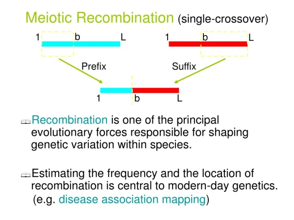
Prefix Suffix Meiotic Recombination(single-crossover) b 1 L 1 b L • Recombination is one of the principal evolutionary forces responsible for shaping genetic variation within species. • Estimating the frequency and the location of recombination is central to modern-day genetics. (e.g. disease association mapping) 1 b L
A Phylogenetic Network 00000 4 00010 a:00010 3 1 10010 00100 5 00101 2 01100 S b:10010 S P 3 4 01101 p g:00101 c:00100 10100 d:10100 f:01101 e:01100
Elements of a Phylogenetic Network (single crossover recombination) • Directed acyclic graph. • Integers from 1 to m written on the edges. Each integer written only once. These represent mutations. • A choice of ancestral sequence at the root. • Every non-root node is labeled by a sequence obtained from its parent(s) and any edge label on the edge into it. • A node with two edges into it is a ``recombination node”, with a recombination point r. One parent is P and one is S. • The network derives the sequences that label the leaves.
Minimizing Recombinations • Any set M of sequences can be generated by a phylogenetic network with enough recombinations, and one mutation per site. This is not interesting or useful. • However, the number of (observable) recombinations is small in realistic sets of sequences. ``Observable” depends on n and m relative to the number of recombinations. • Problem: Given a set of sequences M, find a phylogenetic network generating M, minimizing the number of recombinations. NP-hard (Wang et al 2000, Semple et al 2004)
Minimizing recombinations in unconstrained networks • Problem: given a set of sequences M, find a phylogenetic network generating M, minimizing the number of recombinations used to generate M.
Minimization is an NP-hard Problem There is no known efficient solution to this problem and there likely will never be one. What we do: Solve small data-sets optimally with algorithms that are not provably efficient but work well in practice; Efficiently compute lower and upper bounds on the number of needed recombinations.
Efficient Computation of CloseUpper and Lower Bounds on the Minimum Number of Recombinations in Biological Sequence Evolution Yun S. Song, Yufeng Wu, Dan Gusfield UC Davis ISMB 2005
Computing close lower and upper bounds on the minimum number of recombinations needed to derive M. (ISMB 2005)
Incompatible Sites A pair of sites (columns) of M that fail the 4-gametes test are said to be incompatible. A site that is not in such a pair is compatible.
1 2 3 4 5 Incompatibility Graph a b c d e f g 0 0 0 1 0 1 0 0 1 0 0 0 1 0 0 1 0 1 0 0 0 1 1 0 0 0 1 1 0 1 0 0 1 0 1 4 M 1 3 2 5 Two nodes are connected iff the pair of sites are incompatible, i.e, fail the 4-gamete test. THE MAIN TOOL: We represent the pairwise incompatibilities in a incompatibility graph.
Simple Fact If sites two sites i and j are incompatible, then the sites must be together on some recombination cycle whose recombination point is between the two sites i and j. (This is a general fact for all phylogenetic networks.) Ex: In the prior example, sites 1, 3 are incompatible, as are 1, 4; as are 2, 5.
The grandfather of all lower bounds - HK 1985 • Arrange the nodes of the incompatibility graph on the line in order that the sites appear in the sequence. This bound requires a linear order. • The HK bound is the minimum number of vertical lines needed to cut every edge in the incompatibility graph. Weak bound, but widely used - not only to bound the number of recombinations, but also to suggest their locations.
Justification for HK If two sites are incompatible, there must have been some recombination where the crossover point is between the two sites.
HK Lower Bound 1 2 3 4 5
HK Lower Bound = 1 1 2 3 4 5
More general view of HK Given a set of intervals on the line, and for each interval I, a number N(I), define the composite problem: Find the minimum number of vertical lines so that every interval I intersects at least N(I) of the vertical lines. In HK, each incompatibility defines an interval I where N(I) = 1. The composite problem is easy to solve by a left-to-right myopic placement of vertical lines.
If each N(I) is a ``local” lower bound on the number of recombinations needed in interval I, then the solution to the composite problem is a valid lower bound for the full sequences. The resulting bound is called the composite bound given the local bounds. This general approach is called the Composite Method (Simon Myers 2002).
8 2 2 1 2 1 3 2 The Composite Method (Myers & Griffiths 2003) 1. Given a set of intervals, and 2. for each intervalI,a numberN(I) Composite Problem: Find the minimum number of vertical lines so that everyI intersects atleast N(I) vertical lines. M
Haplotype Bound (Simon Myers) • Rh = Number of distinct sequences (rows) - Number of distinct sites (columns) -1 <= minimum number of recombinations needed (folklore) • Before computing Rh, remove any site that is compatible with all other sites. A valid lower bound results - generally increases the bound. • Generally Rh is really bad bound, often negative, when used on large intervals, but Very Good when used as local bounds in the Composite Interval Method, and other methods.
Composite Interval Method using RH bounds Compute Rh separately for each possible interval of sites; let N(I) = Rh(I) be the local lower bound for interval I. Then compute the composite bound using these local bounds.
Composite Subset Method (Myers) • Let S be subset of sites, and Rh(S) be the haplotype bound for subset S. If the leftmost site in S is L and the rightmost site in S is R, then use Rh(S) as a local bound N(I) for interval I = [S,L]. • Compute Rh(S) on many subsets, and then solve the composite problem to find a composite bound.
RecMin (Myers) • Computes Rh on subsets of sites, but limits the size and the span of the subsets. Default parameters are s = 6, w = 15 (s = size, w = span). • Generally, impractical to set s and w large, so generally one doesn’t know if increasing the parameters would increase the bound. • Still, RecMin often gives a bound more than three times the HK bound. Example LPL data: HK gives 22, RecMin gives 75.
Optimal RecMin Bound (ORB) • The Optimal RecMin Bound is the lower bound that RecMin would produce if both parameters were set to their maximum possible values. • In general, RecMin cannot compute (in practical time) the ORB. • We have developed a practical program, HAPBOUND, based on integer linear programming that guarantees to compute the ORB, and have incorporated ideas that lead to even higher lower bounds than the ORB.
Computing the ORB • Gross Idea: For each interval I, use ILP to find a subset of sites that maximizes Rh over all subsets in interval I. Set N(I) to the found Rh value, and use these values in the Composite Method. • The result is guaranteed to be the ORB. i.e, the bound one would get by using all 2^m subsets in RecMin.
We have moved from doing an exponential number of simple computations (computing Rh for each subset), to solving a quadratic number of (possibly expensive) ILPs. Is this a good trade-off in practice? Our experience - very much so!
How to compute Opt(I) by ILP Create one variable Xi for each row i; one variable Yj for each column j in interval I. All variables are 0/1 variables. Define S(i,i’) as the set of columns where rows i and i’ have different values. Each column in S(i,i’) is a witness that rows i and i’ differ. For each pair of rows (i,i’), create the constraint: Xi + Xi’ <= 1 + ∑ [Yj: jin S(i,i’)] Objective Function: Maximize ∑ Xi - ∑ Yj -1
Alternate way to compute Opt(I) by ILP First remove any duplicate rows. Let N be the number of rows remaining. Create one variable Yj for each column j in interval I. All variables are 0/1 variables. S(i,i’) as before. For each pair of rows (i,i’) create the constraint: 1 <= ∑ [Yj: jin S(i,i’)] Objective Function: Maximize N - ∑(Yj) -1 Finds the smallest number of columns to distinguish the rows.
Two critical tricks Use the second ILP formulation to compute Opt(I). It solves much faster than the first (why?) 2) Reduce the number of intervals where Opt(I) is computed: I If the solution to Opt(I) uses columns that only span interval L, then there is no need to find Opt(I’) in any interval I’ containing L. Each ILP computation directly spawns at most 4 other ILPs. Apply this idea recursively. L
With the second trick we need to find Opt(I) for only 0.5% - 35% of all the C(m,2) intervals (empirical result). Surprisingly fast in practice (with either the GNU solver or CPLEX).
Bounds Higher Than the Optimal RecMin Bound • Often the ORB underestimates the true minimum, e.g. Kreitman’s ADH data: 6 v. 7 • How to derive sharper bound? Idea: In the composite method, check if each local bound N(I) = Opt(I) is tight, and if not, increase N(I) by one. • Small increases in local bounds can increase the composite bound.
Bounds Sharper Than Optimal RecMin Bound • A set of sequences M is called self-derivable if there is a network generating M where the sequence at every node (leaf and intermediate) is in M. • Observation: The haplotype bound for a set of sequences is tight if and only if the sequences are self-derivable. • So for each interval I where Opt(I) is computed, we check self-derivability of the sequences induced by columns S*, where S* are the columns specified by Opt(I). Increase N(I) by 1 if the sequences are not self-derivable.
Self-Derivability Test Solution in O(2^n) time by DP.
Checking if N(I) should be increased by two If the set of sequences is not self-derivable, we can test if adding one new sequence makes it self-derivable. the number of candidate sequences is polynomial and for each one added to M we check self-derivability. N(I) should be increased by two if none of these sets of sequences is self-derivable.
Program HapBound • HapBound –S. Checks each Opt(I) subset for self-derivability. Increase N(I) by 1 or 2 if possible. This often beats ORB and is still practical for most datasets. • HapBound –M. Explicitly examine each interval directly for self-derivability. Increase local bound if possible. Derives lower bound of 7 for Kreitman’s ADH data in this mode.
ILP Compsite method efficiency • Only C(m,2) intervals, but the time for each is more than for the Hap bound. • With tricks we need to solve the ILP for only 0.5% of all the C(m,2) intervals (empirical result). Shockingly fast in practice.
Typical Result With n = 40, m = 100, r = 10 (ms recombination parameter): HK gives 4 Composite Intervals with Hap Bound or CC bound gives 6 Recmin Composite Subsets with Hap Bound and subsets of size up to 20 in windows of size 20: 9 (7 secs) Composite Subsets with Hap Bound and subsets of size up to 30 in windows of size 30: 10 (takes 10 mins on Powerbook G4) ILP Composite gets 10 and takes 1 second on Linux Box.
Example where RecMin has difficulity in Finding the ORB on a 25 by 376 Data Matrix
The Human LPL Data (Nickerson et al. 1998) (88 Sequences, 88 sites) Our new lower and upper bounds Optimal RecMin Bounds (We ignored insertion/deletion, unphased sites, and sites with missing data.)
000 00 00 100 10 10 Empty. One type-3 operation 010 01 01 011 01 History Bound (Myers & Griffiths 2003) M 000 100 010 011 111 • Iterate the following operations • Remove a column with a single 0 or 1 • Remove a duplicate row • Remove any row • History bound: the minimum number of type-3 operations needed to reduce the matrix to empty
Graphical interpretation of history bound (HistB) • Each operation in the history computation corresponds to an operation that deconstructs the optimal, but unknown ARG. • We deconstruct the optimal ARG by removing tree parts as long as possible; then remove an exposed recombination node; repeat. • Removing an exposedrecombination node in the ARG corresponds to a single type-3 operation. So when deconstructing the optimal ARG, the number of recombination nodes = number of type-3 operations. • Since the optimal ARG is unknown, the history bound is the minimum number of type-3 operations needed to make the matrix empty.
a: 00010 b: 10010 4 M c: 00100 3 d: 10100 e: 01100 f: 00101 1 g: 00101 Operations on M correspond to operations on the optimal ARG s p a: 00010 2 c: 00100 b: 10010 d: 10100 2 5 e: 01100 g: 00101 f: 00101
12345 a: 00010 b: 10010 4 c: 00100 3 d: 10100 e: 01100 f: 00101 1 s Type-2 operation p a: 00010 2 c: 00100 b: 10010 d: 10100 2 5 e: 01100 f: 00101
134 a: 001 b: 101 4 c: 010 3 d: 110 e: 010 f: 010 1 s Type-1 operations p a: 001 2 c: 010 b: 101 d: 110 e: 010 f: 010
134 a: 001 b: 101 4 c: 010 3 d: 110 1 Type-2 operations s p a: 001 2 c: 010 b: 101 d: 110
134 a: 001 b: 101 4 c: 010 3 1 Type-3 operation a: 001 c: 010 b: 101 Then three more Type-1 operations fully reduce M and the ARG.
History bound • Initially required trying all n! permutations of the rows to choose the type-3 operations. • The bound can be computed by DP in O(2n) time (Bafna, Bansal). • On datasets where it can be computed, the history bound is observed to be higher than (or equal to) all studied lower bounds (about ten of them). • There is nostatic definition for what the history bound is -- it is only defined by the algorithms that compute it! The work in this part of the talk comes out of an attempt to find a simple static definition.
Later we will discuss another lower bound, the Connected-Component Lower Bound.