Chapter 3: Introduction to SQL
Chapter 3: Introduction to SQL. Overview of The SQL Query Language Data Definition Basic Query Structure Additional Basic Operations Set Operations Null Values Aggregate Functions Nested Subqueries Modification of the Database. History.

Chapter 3: Introduction to SQL
E N D
Presentation Transcript
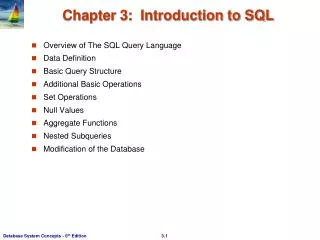
Chapter 3: Introduction to SQL • Overview of The SQL Query Language • Data Definition • Basic Query Structure • Additional Basic Operations • Set Operations • Null Values • Aggregate Functions • Nested Subqueries • Modification of the Database
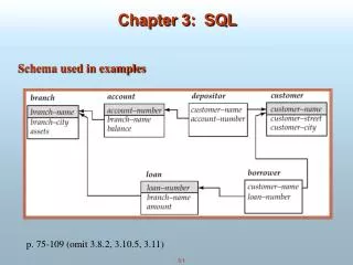
History • IBM Sequel language developed as part of System R project at the IBM San Jose Research Laboratory • Renamed Structured Query Language (SQL) • ANSI and ISO standard SQL: • SQL-86 • SQL-89 • SQL-92 • SQL:1999 (language name became Y2K compliant!) • SQL:2003 • Commercial systems offer most, if not all, SQL-92 features, plus varying feature sets from later standards and special proprietary features. • Not all examples here may work on your particular system.
Data Definition Language Allows the specification of not only a set of relations but also information about each relation, including: • The schema for each relation. • The domain of values associated with each attribute. • Integrity constraints • Security and authorization information for each relation. • The set of indices to be maintained for each relations. • -> physical level • The physical storage structure of each relation on disk. • -> physical level
Domain Types in SQL • char(n). Fixed length character string, with user-specified length n. • varchar(n). Variable length character strings, with user-specified maximum length n. • int.Integer (a finite subset of the integers that is machine-dependent). • smallint. Small integer (a machine-dependent subset of the integer domain type). • numeric(p,d). Fixed point number, with user-specified precision of p digits, with d digits to the right of decimal point.For example, 34.2 is numeric(3,1). • real, double precision. Floating point and double-precision floating point numbers, with machine-dependent precision. • float(n). Floating point number, with user-specified precision of at least n digits. • More are covered in Chapter 4.
Create Table Construct • An SQL relation is defined using thecreate tablecommand: create table r (A1D1, A2D2, ..., An Dn,<integrity-constraint1>, ..., <integrity-constraintk>); • r is the name of the relation • each Ai is an attribute name in the schema of relation r • Di is the data type of values in the domain of attribute Ai • Example: create tableinstructor (IDchar(5),name varchar(20) not null,dept_name varchar(20),salarynumeric(8,2)); • insert into instructor values (‘10211’, ’Smith’, ’Biology’, 66000); • 字串加單引號 • insert into instructor values (‘10211’, null, ’Biology’, 66000); ->wrong! • insert into instructor values (‘10211’, ’Smith’, ’Biology’, null); ->right!
Integrity Constraints in Create Table • not null • primary key (A1, ..., An ) • foreign key (Am, ..., An ) references r Example: Declare ID as the primary key for instructor. create tableinstructor (IDchar(5),name varchar(20) not null,dept_name varchar(20),salarynumeric(8,2),primary key (ID),foreign key (dept_name) references department); primary key declaration on an attribute automatically ensures not null
And a Few More Relation Definitions • create tabledepartment (dept_namevarchar(20),buildingvarchar(15),budgetnumeric(12, 2), primary key (dept_name)); • create tableteaches (IDvarchar(5),course_idvarchar(8),sec_idvarchar(8),semestervarchar(6),yearnumeric(4,0), primary key (ID, course_id, sec_id, semester, year),foreign key (ID) references instructor,foreign key (course_id, sec_id, semester, year) references section); Note: 1. A primary key can consist of many attributes. 2. A table can have many foreign keys.
Drop and Alter Table Constructs • drop table command deletes all information about the dropped relation from the database. • 如果只刪除資料而不刪除定義的話,請使用delete語法. • alter table command is used to add attributes to an existing relation: • alter table r add A D; • where A is the name of the attribute to be added to relation r and D is the domain of A. • All tuples in the relation are assigned null as the value for the new attribute. • alter table r drop A; • where A is the name of an attribute of relation r
Relational Schemas • instructor (ID, name, dept_name, salary) • teaches (ID, course_id, sec_id, semester, year) • course (course_id, title, dept_name, credits) • section (course_id, sec_id, semester, year, building, room_number, time_slot_id) • student (ID, name, dept_name, tot_cred) • takes (ID, course_id, sec_id, semester, year, grade) • department (dept_name, building, budget)
Relational Instances • section • course
More Relational Instances • department • teaches • instructor
Basic Query Structure • A typical SQL query has the form:select A1, A2, ..., Anfromr1, r2, ..., rmwhere P; • Ai represents an attribute • Ri represents a relation • P is a predicate. • The result of an SQL query is a relation. • Note: An SQL query is usually ended with the semicolon “;”, but it might vary in different software or different programming languages. (For example, 在ASP.net程式中要加.)
The select Clause • The select clause list the attributes desired in the result of a query • corresponds to the projection operation of the relational algebra • Example: find the names of all instructors:( 參照instance) select namefrom instructor; • NOTE: SQL names are case insensitive (i.e., you may use upper- or lower-case letters.) • E.g., Name ≡ NAME ≡ name • Some people use upper case wherever we use bold font.
The select Clause (Cont.) • SQL allows duplicates in relations as well as in query results. To force the elimination of duplicates, insert the keyword distinctafter select. • Find the department names of all instructors, and remove duplicates select distinct dept_namefrom instructor; • An asterisk in the select clause denotes “all attributes” select *from instructor; • The select clause can contain arithmetic expressions involving the operation, +, –, , and /, and operating on constants or attributes of tuples. • The following query would return a relation that is the same as the instructor relation, except that the value of the attribute salary is divided by 12. selectID, name, salary/12from instructor; <- A query can have no “where”.
The where Clause • The whereclause specifies conditions that the result must satisfy • Corresponds to the selection predicate of the relational algebra. • To find all instructors in Comp. Sci. dept with salary > 70000 select namefrom instructorwhere dept_name =‘Comp. Sci.'and salary > 70000; • Comparison results can be combined using the logical connectives and, or, and not. • Comparisons can be applied to results of arithmetic expressions. • 注意: • 字串用單引號 • 不等於是用 <>
The from Clause • The fromclause lists the relations involved in the query • Corresponds to the Cartesian product operation of the relational algebra. • Find the Cartesian product instructor X teaches select from instructor, teaches; • generates every possible “instructor – teaches” pair, with all attributes from both relations. • Cartesian product not very useful directly, but useful combined with where-clause condition (selection operation in relational algebra).
Cartesian Product teaches instructor
Joins • For all instructors who have taught courses, find their names and the course ID of the courses they taught. select name, course_idfrom instructor, teacheswhere instructor.ID = teaches.ID; • Find the course ID, semester, year and title of each course offered by the Comp. Sci. department (參照instance) select section.course_id, semester, year, titlefrom section, coursewhere section.course_id = course.course_id anddept_name = ‘Comp. Sci.‘; • Join: Cartesian product + 限制式 • PS. 相同屬性出現在兩個以上的表格,前面必須加註 來源表格
Try Writing Some Queries in SQL • Find the titles of courses in the Comp. Sci. department that have 3 credits. Answer: • Find the course_ids and sec_ids which were offered by an instructor named “Einstein”; make sure there are no duplicates in the result. Answer:
Natural Join • Natural join matches tuples with the same values for all common attributes, and retains only one copy of each common column • 注意:common attributes通常是primary key或foreign key • select *from instructor natural join teaches; <- 有些軟體不支援此語法!
Natural Join (Cont.) • Danger in natural join: unrelated attributes with same name which get equated incorrectly • Example: List the names of instructors along with the titles of courses that they teach • Incorrect version (equates course.dept_name with instructor.dept_name) select name, titlefrom instructor natural join teaches natural join course; <- 錯誤的原因在於instructor和course不用同一系! • Correct version select name, titlefrom instructor natural join teaches, coursewhere teaches.course_id= course.course_id; <-在from裡使用逗號”,”,所以course是和前一個combined relation做cartesian product. • 注意:大部分軟體所支援的join語法會在第四章補充。
The Rename Operation • The SQL allows renaming relations and attributes using the as clause: old-name as new-name • “as”放在select clause: • select ID, name, salary/12 as monthly_salaryfrom instructor; • Note: “as” 是在最後做,所以新定義的屬性名稱不能用在query其他地方 • Tuple variables: “as”放在from clause • Usually used to compare tuples in the same relation. • Example: Find the names of all instructors who have a higher salary than some instructor in ‘Comp. Sci’. (see the next page) • select distinct T. namefrom instructor as T, instructor as Swhere T.salary > S.salary and S.dept_name = ‘Comp. Sci.’; • Keyword as is optional and may be omittedinstructor as T ≡ instructorT
Example of Tuple Variables instructor S T
String Operations • SQL includes a string-matching operator for comparisons on character strings. The operator “like” uses patterns that are described using two special characters: • percent (%). The % character matches any substring. (* in OS) • underscore (_). The _ character matches any character. (? in OS) • Find the names of all instructors whose name includes the substring “dar”. select namefrom instructorwherename like '%dar%'; • SQL supports a variety of string operations such as • concatenation (using “||”) • converting from upper to lower case (and vice versa) • finding string length, extracting substrings, etc.
Ordering the Display of Tuples • List in alphabetic order the names of all instructors select distinct namefrom instructororder by name; (c.f. page 3.13) • We may specify desc for descending order or asc for ascending order. For each attribute, ascending order is the default. • Example: order bynamedesc • Can sort on multiple attributes • Example: order by dept_name, name
Where Clause Predicates • SQL includes a between comparison operator • Example: Find the names of all instructors with salary between $90,000 and $100,000 (that is, $90,000 and $100,000) • select namefrom instructorwhere salary between 90000 and 100000; It is equivalent to select namefrom instructorwhere salary>=90000 and salary <= 100000;
Duplicates • Recall that the relational algebra operators support the set semantics. • Multisetversions of some of the relational algebra operators: • given multiset relations r1 and r2: 1. (r1): If there are c1 copies of tuple t1 in r1, and t1 satisfies selections ,, then there are c1 copies of t1 in (r1). 2. A (r ): For each copy of tuple t1in r1, there is a copy of tupleA (t1) in A (r1) where A (t1) denotes the projection of the single tuple t1. 3. r1 x r2: If there are c1 copies of tuple t1in r1 and c2 copies of tuple t2 in r2, there are c1 x c2 copies of the tuple t1. t2 in r1 x r2 • Example: Suppose multiset relations r1 (A, B) and r2 (C) are as follows: r1 = {(1, a) (2,a)} r2 = {(2), (3), (3)} • Then B(r1) would be {(a), (a)}, while B(r1) x r2 would be {(a,2), (a,2), (a,3), (a,3), (a,3), (a,3)}
Duplicates (Cont.) • SQL duplicate semantics: select A1,, A2, ..., Anfrom r1, r2, ..., rmwhere P is equivalent to the multiset version of the expression: • Example: • See page 3.13 for example of projection
Set Operations • Find courses that ran in Fall 2009 or in Spring 2010 (selectcourse_id from section where sem = ‘Fall’ and year = 2009)union(selectcourse_id from section where sem = ‘Spring’ and year = 2010); • Find courses that ran in Fall 2009 and in Spring 2010 (selectcourse_id from section where sem = ‘Fall’ and year = 2009)intersect(selectcourse_id from section where sem = ‘Spring’ and year = 2010); • Find courses that ran in Fall 2009 but not in Spring 2010 (selectcourse_id from section where sem = ‘Fall’ and year = 2009)except(selectcourse_id from section where sem = ‘Spring’ and year = 2010);
Set OperationExample union intersect except
※ Duplicates of Set Operations • Set operations union, intersect, and except • Each of the above operations automatically eliminates duplicates. -> support the set semantics. • To retain all duplicates, use the corresponding multiset version syntax: • union all, intersect alland except all. • Suppose a tuple occurs m times in r and n times in s, then, it occurs: • m + n times in r union all s • min(m,n) times in rintersect all s • max(0, m – n) times in rexcept all s • Example: A = {p, p, q}, B = {p, r} • A union all B = {p, p, p, q, r}; A union B = {p, q, r} • A intersect all B = {p} • A except all B = {p, q}; B except all A = {r}
Null Values • It is possible for tuples to have a null value, denoted by null, for some of their attributes • null signifies an unknown value or that a value does not exist. • The result of any arithmetic expression involving null is null • Example: 5 + null returns null • The predicate is null can be used to check for null values. • Example: Find all instructors whose salary is null. select namefrom instructorwhere salary is null;
Null Values and Three Valued Logic • Any comparison with null returns unknown • Example: 5 < null or null <> null or null = null • Three-valued logic using the truth value unknown: • OR: (unknownortrue) = true, (unknownorfalse) = unknown (unknown or unknown) = unknown • AND: (true and unknown) = unknown, (false and unknown) = false, (unknown and unknown) = unknown • NOT: (not unknown) = unknown • Result of where clause predicate is treated as false if it evaluates to unknown • Example: • Select C from T1 where A = ‘’ and B = ‘’ -> {7} • Select C from T1 where A = ‘’ or B = ‘’ -> {8, 7} A B C 8 7 T1
Aggregate Functions • These functions operate on the multiset of values of a column of a relation, and return a value avg: average valuemin: minimum valuemax: maximum valuesum: sum of valuescount: number of values A B C • Example: sum(c ) 7 7 3 10 27
Aggregate Functions (Cont.) • Find the average salary of instructors in the Computer Science department (see page 3.10) • select avg (salary)from instructorwhere dept_name= ’Comp. Sci.’; • Find the number of tuples in the course relation • select count (*)from course; • Find the total number of instructors who teach a course in the Spring 2010 semester • select count (distinct ID)from teacheswhere semester = ’Spring’ and year = 2010;
Aggregate Functions – Group By • Find the average salary of instructors in each department • select dept_name, avg (salary) as avg_salaryfrom instructorgroup by dept_name; avg_salary
Aggregation (Cont.) • Note: Attributes in select clause outside of aggregate functions must appear in group by list <-否則會出現multi-valued的狀況,違反 atomic的限制 • /* erroneous query */select dept_name, ID, avg (salary)from instructorgroup by dept_name • Find the number of instructors in each department who teach a course in the Spring 2010 semester. dept_name ID avg(salary) 72000 77333 ………. biology Comp. Sci ….. 76766 45565 10101 83821 ….. select dept_name, count (distinctID) as instr_countfrom instructor natural join teacheswhere semester= ‘Spring’ and year = 2010group by dept_name; (參照join結果)
Aggregate Functions – Having Clause • Find the names and average salaries of all departments whose average salary is greater than 42000 select dept_name, avg (salary) from instructor group by dept_name having avg (salary) > 42000; (參照分群結果) Note: predicates in the having clause are applied after the formation of groups whereas predicates in the where clause are applied before forming groups • 注意: • aggregate function 不能直接使用在where clause裡. • 放在having和select clause裡的aggregate function 可不同
Aggregate Functions – Example • For each course section offered in 2009, find the average total credits (tot_cred) of all students enrolled in the section, if the section had at least 2 students. select course_id, semester, year, sec_id, avg (tot_cred)from takes natural join student where year = 2009 group by course_id, sec_id, semester, yearhaving count(ID) >= 2;
Practice • Find the number of instructors in each department. • Find the names of all departments whose instructors are more than 10.
Null Values and Aggregates • Total all salaries select sum (salary )from instructor; • Above statement ignores null amounts • Result is null if there is no non-null amount • All aggregate operations except count(*) ignore tuples with null values on the aggregated attributes • What if collection has only null values? • count returns 0 • all other aggregates return null ID name salary 10101 12121 15151 22222 32343 Srinivasan Wu Mozart Einstein El Said 40000 null 75000 75000 null
Nested Subqueries • SQL provides a mechanism for the nesting of subqueries. • A subquery is a select-from-where expression that is nested within another query. • A common use of subqueries is to perform tests for set membership, set comparisons, and set cardinality.
Example Query • Find courses offered in Fall 2009 and in Spring 2010 (另一種寫法) select distinct course_id from section where semester = ’Fall’ and year= 2009 and course_id in (select course_id from section where semester = ’Spring’ and year= 2010); • Find courses offered in Fall 2009 but not in Spring 2010 select distinct course_id from section where semester = ’Fall’ and year= 2009 and course_id not in (select course_id from section where semester = ’Spring’ and year= 2010); • 練習題:Find courses offered in Fall 2009 orin Spring 2010
Set Comparison • Find names of instructors with salary greater than that of some (at least one) instructor in the ‘Comp. Sci’ department. select distinct T.name from instructor as T, instructor as S where T.salary > S.salary and S.dept_name = ’Comp. Sci’ • Same query using > some clause select name from instructor where salary > some (select salary from instructor where dept_name = ’Comp. Sci’) • 確定sub-query只輸出一筆資料則可省略量詞some或all.
0 5 6 Definition of Some Clause • F <comp> some r t r such that (F <comp> t )Where <comp> can be: <= <> (5 < some ) = true (read: 5 < some tuple in the relation) 0 (5 < some ) = false 5 0 ) = true (5 = some 5 0 (5 some ) = true (since 0 5) 5 (= some) in However, ( some) not in
Example Query • Find the names of all instructors whose salary is greater than the salary of all instructors in the Biology department. select name from instructor where salary > all (select salary from instructor where dept_name = ’Biology’) • 練習題:Find the names of all instructors whoearn the most salary in the Biology department. • Answer:
0 5 6 Definition of all Clause • F <comp> all r t r (F <comp> t) (5 < all ) = false 6 ) = true (5 < all 10 4 ) = false (5 = all 5 4 ) = true (since 5 4 and 5 6) (5 all 6 (all) not in However, (= all) in
Test for Empty Relations • The exists construct returns the value true if the argument subquery is nonempty. • exists r r Ø • not exists r r = Ø
Correlation Variables • Another way of specifying the query “Find all courses taught in both the Fall 2009 semester and in the Spring 2010 semester” select course_idfrom section as Swhere semester = ’Fall’ and year= 2009 and exists (select *from section as Twhere semester = ’Spring’ and year= 2010 and S.course_id= T.course_id); • S: correlation variable, or correlation name • Correlated subquery: a subquery in the where clause that uses a correlation variable from an outer query • 注意:有的subquery需要額外宣告變數,有的不需要 (see page 3.43).