Download

1 / 45
480 likes | 673 Vues
Jiang-Tao Su and Hong-Qi Zhang National Astronomical Observatories Chinese Academy of Sciences. Measurements of Vector Magnetic Fields. Outline. Foundation for measuring of vector magnetic fields ----Zeeman effect Magnetogram data reduction Calibrations for vector magnetic fields

E N D
Jiang-Tao Su and Hong-Qi Zhang National Astronomical Observatories Chinese Academy of Sciences Measurements of Vector Magnetic Fields
Outline • Foundation for measuring of vector magnetic fields ----Zeeman effect • Magnetogram data reduction • Calibrations for vector magnetic fields and Faraday rotation • Influence of stray-light on longitudinal magnetic signal
I. Zeeman effect Intensity differences of Zeeman splitting polarized components diagnosed by magnetographs are Stokes I、Q、U、V. The relationships among them as the followings: Stokes V ---- BL Stokes Q ---- BT
Diagnosis of Stokes parameters Q/I, U/I, V/I by Video Vector Magnetograph at Huairou With line FeIλ5324.19 Å Longitudinal magnetic fieldBL 0.0 Å Calibrated Calibrated Transverse magnetic field BT Q/I V/I 0.0 Å -0.075 Å U/I (Zhang 2000)
1、Linear bias present in Stokes Q/I and U/I II. Magnetogramdata reduction Estimate of bias in areas outside the AR -0.12 Å -0.12 Å
Distribution plots of the U/I and Q/I I intensities Transverse field bias distribution Subtract linear biases from original Stokes Q/I and U/I data:
2、Circular-to-linear cross talk Measurements of transverse magnetic fields with filter tuned to line wings are to be suffered the affections of cross-talk between circular and linear polarized lights. Measurements of transverse magnetic fields with filter tuned to line center are to be suffered the more serious affections of Faraday rotations
The cross-talk is estimated by making a scatter plot of the difference between the red (r) and blue (b) wings [(Qb-Qr)/I vs. (Vb-Vr)/I, and (Ub-Ur)/I vs. (Vb-Vr)/I] at the ±60 mÅ filter positions, respectively, over the entire field of view. b: -0.06Å r: +0.06Å
Before the cross-talk corrections The formulae for correction of cross-talk: Two azimuths observed at ±120mÅ from the line center After the cross-talk corrections
The line of FeIλ5324.19 Å in umbra region A explanation for magnitude differences in sunspot umbra region is: There is the asymmetry in two wings of line FeIλ5324.19 Å in umbra region A rough ratio of polarized signal Q or U at 150mÅ red to at 150mÅ blue is 1.5, estimated from the line of FeIλ5324.19 Å.
III. Calibrations of full vector magnetic fields and Faraday rotation Calibrationmethod: With nonlinear least-square techniques, the observed Stokes V/I, Q/I and U/I profiles were compared with the model profiles and the parameters of magnetic strength H, inclination γ and azimuth χ were obtained. Then we got the coefficients of CL and CT for longitudinal and transverse components of magnetic field by the approximate relations: BL=CL(V/I),BT=CT [(Q/I)2+(U/I) 2] 1/4.
Preceding calibration works • Theoretical calibrations of vector magnetic fields (Ai, Li and Zhang, 1982) • Empirical calibration by comparison with Kitt Peak data (Ai, 1994-1995) • Calibration of longitudinal magnetic field with observational and empirical methods using Huairou data (Wang, Ai and Deng, 1996)
Observed data (Stokes profiles) The Stokes profiles data were obtained on 2002-10-24 and 2003- 10-23, with the HSOS vector magnetograph for two relative simple sunspots of AR 10162 (N26 E04) and AR 10484 located (N04 E12.4). The former data are used to diagnose the Faraday rotation the latter data to calibrate vector magnetic fields. The spectral scan data were Stokes images extending from 150mÅ in the blue wing to +150mÅ in the red wing of the FeIλ5324.19 Å line at steps of 10mÅ. The standard deviation data were Stokes images observed at ±60mÅ from the line center.
Analytical solutions for Stokes parameters Landolfi & Landi Del’Innocenti (1982)
Definition for : All parameters being treated as independent parameters (Balasubramaniam and West 1991).
Map of the sunspot’s filtergram showing radii and circles for the selection of the pixels used in the analysis (Hagyard, et al. 2000). Azimuth rotation >60º * * Sunspot filtergram of AR 10162 * * Azimuth rotation about 40º * * * * * *
Q/I U/I AR 10162 V/I =0.5actan(Q/U) The 8 parameters obtained are as the followings:
Q/I U/I V/I a b AR 10484 c d
Some abnormal pixels as the minus Doppler width obtained are deleted in data reduction.
Calibration of transverse field: Calibration of longitudinal field: Calibrations at line wing -0.12Å Calibrations at the routine observational line positions Calibration of transverse field: Calibration of longitudinal field:
Discussions Least-square fitting: Virtues: more accurate total magnetic field strength, declination and azimuth of magnetic field vector can be obtained. Shortcomings: (1)only the strong fields of sunspots can be derived (during the process of data reduction, we get the minimum transverse magnetic field strength 220 Gauss, the minimum longitudinal magnetic field strength 49 Gauss). (2) the process of obtaining the data is time-consuming. The fitting errors for a sampled pixel
Faraday rotation Azimuth of magnetic field 1/2tg-1(U’/Q’) Orientations of three linearly polarized components (nбL,nπ, nбR) 1/2tg-1(U’/Q’) Relative retardation Propagation Faraday rotation Top of solar atmosphere Azimuth difference Δ =ф-ф’ Rotation of polarization direction Orientations of three linearly polarized light (nбL,nπ, nбR) 1/2tg-1(U/Q) Diagnostic of magnetograph
Hagyard, et al. (2000) found that Faraday rotation of azimuth will be a significant problem in observations taken near the center of a spectral line for fields as low as 1200 G and inclinations of the fields in the range of 20 º ~ 80 º degree. Bao, et al. (2000) and Zhang (2000) found a mean azimuth rotation only ~12 º for Huairou transverse field data taken at the center of FeIλ5324.19 Å. Zhang, et al. (2003), by comparisons of the datafrom Huairou, Mees and Mitaka observatories, found that there is a basic agreement on the transversal fields. Why is there such controversy on azimuth rotation? A controversy on Faraday rotation
B= 1500 G,γ=30o,χ=22.5o Azimuth ф Wavelength π-σ rotation effect The linearly polarized component at line center is perpendicular to the direction of the linearly polarized component in the wings.The azimuth will abruptly change 900 obtained with different positions of a spectral line from line wings to line center. We cannot separate the two effects (Hagyard et al. 2000). So the combination effect of them affects the measurements of azimuth of magnetic field vector.
4. Elimination of 180º ambiguity =0.5actan(Q/U) π-σ rotation eliminated partially byconvolution withfilter profile 1.、2. π-σ rotation 3.π-σand Faraday rotations
A deduction about azimuth rotation • The spectral line with a relatively larger Landé factor g has the more possibility to confront “splitting” enlarged due to π-σ rotation effect • The Landé factor g of line FeIλ5324.19 Å is 1.5 and FeIλ5250.22 Å 3. Thus, the former will confront less large (say, > 60º) azimuth rotation
Definition of azimuth rotation: AR 10162
Azimuth rotation >60º About 40º Azimuth rotation >60º Azimuth rotation about 40º
The results show that the rotation of azimuth is less significant in the observations taken near the center of the Fe I 5324.19Å line than those taken near the center of the Fe I 5250.22 Å line.
VI.Influence of stray-light on longitudinal magnetic signal • Observational phenomenon Magnetic signal V/I in umbra center is weaker than that of penumbra. The causes may be: (1) Stray light disturb polarized light. (2) There is serious magnetic saturation effect when measuring magnetic fields in the center of sunspot. (3) There is CCD nonlinear response to weaker polarized light intensity.
Numerical simulation of magnetic saturation Employed different solar atmosphere model,the theoretical calibrating curve for longitudinal magnetic field (LMF) can be obtained at -0.75 Å from line center. Linear deviation for LMF calibration
Numerical simulations show that when BL = 3000 G, the saturation effect can only cause a maximum error of ~ 6% for the band-pass position of -0.075 Å to the center of Fe Iλ5324.19 Å. Moreover, in umbra region, Stokes V/I profiles are approximately complete and not distorted.
So magnetic saturation effect is not the main contributor to this phenomena. • Stray light Stray light include two parts (Martinez Pillet 1992; Chae et al. 1998): (1) small-spread-angle (SSA) stray light (also named blurring part) caused by atmospheric seeing (affecting scale: several arcsecs) . (2) large-spread-angle (LSA) stray light (also named scattering part) originating from the instrument and the Earth’s atmosphere (affecting scale: larger than 10 arcsecs). The observational Stokes I obs image result from spatial re-distributions of disturbance-free Stokes I image : A point-spread-function (PSF) (SSA part and LSA part) is taken as in the form:
the limb So the observed Iobs can be rewritten: Фj Фj ФL
Accurate determination of the solar limb • Methods of PSF and LSA stray light correcting curve determinations Aureole data Stokes I image Derivative of I with respect to distance
We make a linear least-square fit to the aureole data and the chi-square is defined as: Intensity profile across the limb LSA stray light integral (correcting curve)
Variation of scattered light fraction in a day Polynomial fit Ruan Guiping (2004)
Large-spread-angle stray light correction In routine observations, what we should first is to subtract stray light intensity from polarized light intensity, which should be large-spread-angle stray light. The intensity to be subtracted is named as BLACK LEVEL (BL). However, it is clear that the stray light intensity near an active region (AR) is not equal to that of Sun limb. The intensities of left and right circularly polarized light versus pixel location. IS refers to the actual background noise signal. Ii is a series of BL intensities and i = 1, 2, 3, 4, and 5.
The magnetic signal V/I can be expressed as: Where IR and IL are right and left circularly polarized light intensities, IRS and ILS are right and left circularly polarized background noise intensities. (1)Stokes V/I is smaller than the real value. (2)Stokes V/I is nearly equal to the real value. (3)Stokes V/I is larger than the real value. In practice, how to select a reasonable BL to make:
Correction method of large-spread-angle stray light The observed sunspot was located r=0.5 from solar disk center. The intensity ratio between distance from disk center r=1. and r=0.5 is 1.93. We also know BL= 65 in the limb. So The BL value (r=0.5) can be obtained from this expression: Where L zero≈110 (the position stray light signal is zer0). Then BL (r=0.5) is 43. The magnetograms for BL of 40, 55 and 65 are:
Affection of strayed light on magnetic field azimuths noise signal introduced by strayed light