Download
1 / 20
200 likes | 358 Vues
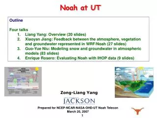
Noah at UT. Outline Four talks Liang Yang: Overview (20 slides) Xiaoyan Jiang: Feedback between the atmosphere, vegetation and groundwater represented in WRF/Noah (27 slides) Guo-Yue Niu: Modeling snow and groundwater in atmospheric models (83 slides)

E N D
Noah at UT • Outline • Four talks • Liang Yang: Overview (20 slides) • Xiaoyan Jiang: Feedback between the atmosphere, vegetation and groundwater represented in WRF/Noah (27 slides) • Guo-Yue Niu: Modeling snow and groundwater in atmospheric models (83 slides) • Enrique Rosero: Evaluating Noah with IHOP data (9 slides) Zong-Liang Yang Prepared for NCEP-NCAR-NASA-OHD-UT Noah Telecon March 20, 2007
Model Development at UT-Austin (http://www.geo.utexas.edu/climate/Research/publications.htm) • Improved TOPMODEL runoff (Yang and Niu, 2003, GPC; Niu and Yang, 2003, GPC; Niu et al., 2005, JGR) • Improved frozen soil scheme (Niu and Yang, 2006, JHM) • Multi-layer snow (Yang and Niu, 2003, GPC) • Snow and vegetation canopy interaction (Niu and Yang, 2004, JGR) • Snow cover fraction (Niu and Yang, 2007, JGR) • Global unconfined aquifer/groundwater component (Niu et al., 2007, JGR) • Comparison of stochastic and physically-based subgrid snow cover fraction for snow assimilation (Su et al., 2007; Yang et al., 2007) These physical parameterizations are expected to work for both climate and weather models.
Noah @ UT • To put a dynamic vegetation and groundwater component in the Noah LSM • understand the feedback mechanisms between precipitation, soil moisture, and vegetation/groundwater dynamics • To improve weather and climate forecasts on time scales from hourly to seasonal (Jiang et al., 2007a, in preparation; Yang et al., 2007, in preparation) • To interpret and transfer weather and climate forecasts for water resources management applications • To put a biogenic VOC emission component in the Noah LSM • understand the impacts of climate change and land use/land cover change on BVOC emissions and the formation of near ground ozone (Gulden and Yang, 2006, Atmospheric Environment; Jiang et al., 2007b, in preparation)
The Modeling Domains: Multiple interactive nesting grids: Weather Research and Forecast (WRF) Model, version 2.02 (http://www.wrf-model.org/) The model is developed by NCAR, NCEP and Universities. 30 km grid; 31 Levels Temperature, wind, humidity, pressure predicted 3-10 km grid; 31 Levels Temperature, wind, humidity, pressure predicted 90 km grid; 31 Levels Temperature, wind, humidity, pressure prescribed from large-scale analyses
Vegetation Distribution in the Model Other Land Data: Vegetation LAI Albedo Roughness length Stomatal parameters Soil Topography Validation: Weather stations Hydrologic stations Remote sensing Field data
Stomatal Conductance in Noah • Transpiration parameterized through surface conductance based on the model of Jarvis (1976). For a single leaf:
Noah with Modifications (1) The ability of roots to uptake soil water depends on the availability of soil water. In Noah, this is a linear function, which may work if soil is near saturated. We make it a step-function, guided by observations. We call the experiment Noah SWF (soil water factor).
Role of Land Surface Processes in Modulating NAMS Rainfall OBS WRF/SLAB WRF/NOAH WRF/NOAH SWF JUN JUL AUG WRF/SLAB fails to produce rainfall for June thru August. WRF/Noah fails to capture rainfall in August. WRF/Noah-SWF captures rainfall in August.
Noah with Modifications (2) • Noah prescribes fractional green vegetation. • In the real world, vegetation growth depends on precipitation, temperature, nutrients, and others. • This can be modeled by • Relating stomatal conductance to photosynthesis & environmental conditions, and • Allocating assimilated carbon to leaves, stem, wood, and roots.
Leaf Anatomy Stomate (pl. stomata)
Carbon and Water • Plants eat CO2 for a living • They open their stomata to let CO2 in • Water gets out as an (unfortunate?) consequence • For every CO2 molecule fixed about 400 H2O molecules are lost
Photosynthesis and Conductance Stomatal conductance is linearly related to photosynthesis: (The “Ball-Berry-Collatz” parameterization) RH at leaf sfc photosynthesis stomatalconductance CO2 at leaf sfc Photosynthesis is controlled by three limitations(The Farquahar-Berry model): Enzyme kinetics(“rubisco”) Light Starch
Comparison of Observed & Simulated Rainfall OBS WRF/Noah SWF WRF/Noah DV JUN JUL AUG
Conclusions • Strong sensitivity to land surface processes • SLAB (without vegetation) fails to simulate the monsoon rainfall in all months • Noah (with prescribed vegetation) is better, but under-estimates the August rainfall • Noah (with improved root water uptake and response) is even better • Noah (with improved carbon and water coupling and leaf’s dynamic response to rainfall) gives the best overall simulation of the warm season rainfall • In the southern monsoon regions • In the southern Great Plains. • Dynamic vegetation has the largest impacts on the simulation of rainfall in the SGP, which is the area that shows the largest memory to soil moisture conditions.
Groundwater In LSMs without groundwater, water is NOT conserved over irrigated areas. With our simple aquifer scheme added to LSM, we could more realistically model • Agriculture (irrigation) • Water resources (pumpage, river flow)
Representing Irrigation in CLM-GW Case Study: High Plains Aquifer Data courtesy of B. Scanlon
Representing Irrigation in CLM-GW Pumpage≥ΔET (wet season) Pumpage≤ΔET (dry season)
PILPS-GW:Project for Intercomparison of Land Surface Parameterizations: Groundwater Objective: Improve LSM subsurface hydrology Interested to become a contributor? Please contact Lindsey Gulden gulden@mail.utexas.edu; 812-603-3873 Zong-Liang Yang liang@mail.utexas.edu; 512-471-3824 Gulden et al.,2007, GRL (submitted)
Conclusions • We have developed schemes for topography-based runoff, frozen soil, interactive vegetation, groundwater, and sub-grid-scale variability of snow cover. • An LSM augmented with above treatments simulates better terrestrial water storage dynamics across a wide range of spatial scales (see Niu’s talk) • An LSM with a groundwater component makes it logical to deal with irrigation through pumpage rates. • The augmented LSMs (Noah), when operated in the coupled mode, can improve the simulations of near-surface climate variables (see Jiang’s talk) • Parameter estimation and calibration is important to guide the model development (see Rosero’s talk).