Download
1 / 12
120 likes | 314 Vues
Effort Discounting of Exam Grades. Heidi L. Dempsey, David W. Dempsey, & Arian Ward Jacksonville State University.

E N D
Effort Discounting of Exam Grades Heidi L. Dempsey, David W. Dempsey, & Arian Ward Jacksonville State University
The study of temporal discounting of rewards—the tendency to prefer a smaller, sooner reward over a larger, later reward—has been one of the topics examined in the greatest depth in the behavioral economics literature, with probability discounting of rewards—the tendency to prefer rewards that have a higher probability of occurring—following close behind. However, both of these constructs refer to rewards that are received in cases where the participant has put forth no effort. Except for cases such as investment or gambling, little comes to us without effort. One area that has received less empirical study is the domain of effort discounting (e.g, Silva & Gross, 2004). One reason for this may be because effort and time are confounded. This is especially true in education, where students must actively engage in reading and comprehending course material in order to receive a high score. But, even though time and effort are inexorably intertwined in the education field, people can be asked to make a decision about where their indifference point lies with regard to how much effort/time they would be willing to expend in order to receive differing exam grades. The purpose of the present study was to examine whether students would discount exam grades in a hyperbolic-like manner, showing the same type of discounting curve found in temporal and probability discounting, and to correlate exam discounting with the discounting of monetary rewards.
Method • Participants • Two data sets were used. First is referred to as “Spring 2012” and there were 209 participants who ranged in age from 18 to 54 years old, with a mean age of 22.6 years. The majority were freshman and 62% of the students were female. • The second data set was collected during several semesters in 2011 and 2012 (hereafter referred to as “2011-2012”). This sample consisted of 318 participants who ranged in age from 18 to 56 years old, with a mean age of 22.7. Again, the majority were freshman and 62% of the participants were females. • Materials and Procedure • Participants completed an online survey in exchange for course credit. Several personality scales were included along with some individual difference measures, but they are not included in the current analysis. Measures that are included in the analysis are described below.
Exam Discounting Measure • Participants were asked a series of questions which were identical in wording, with the exception that the maximum number of hours required to study to receive 100% was altered to be 1, 2, 3, 4, 7, 10, 15, 21, 30, or 45 hours. The last three hour maximums were added because students in previous studies did not discount enough when the maximum was shorter. The three hour scenario is reproduced here: • Imagine that you were enrolled in a JSU course where you could study for **3 hours** and receive 100% on the exam. However, if you choose to study for less time, you would receive a lower exam grade. The list of exam grades and corresponding study times are listed below. • 100% in 3 hrs 85% in 2 hrs 56% in 1 hr 0% in 0 min97% in 2 hrs 45 min 80% in 1 hr 45 min 46% in 45 min94% in 2 hrs 30 min 73% in 1 hr 30 min 33% in 30 min90% in 2 hrs 15 min 65% in 1 hr 15 min 18% in 15 min • The scaling of choices was based on the standard learning curve, such that even a little studying will result in substantially increased grades, whereas it takes a great deal of studying to receive the highest possible grade (e.g., Ettlinger, 1926; Mazur & Hastie, 1978). For the purposes of this study, the learning curve was modified so that the maximum reward was actually attainable. The scaling is referred to as “logarithmic” because the shape of the curve roughly approximates a logarithmic curve (increasing, concave down).
Monetary Choice Questionnaire • The Monetary Choice Questionnaire (MCQ; Kirby, Petry & Bickel, 1999) was developed to give researchers an easy-to-administer pencil-and-paper measure of delayed discounting of monetary rewards. The 27 items ask participants to choose whether they would take a given dollar amount of money right now, or if they would prefer to wait for the maximum amount. Each of these questions was designed to correspond to a different k-value (the measure of discounting rate) based on a hyperbolic discounting curve (Mazur, 1987). Thus, by following Kirby’s (2000) manual for inputting the data in Excel, you can estimate the discounting rate for each participant for small, medium, and large dollar amounts. Sample questions: • Would you prefer $69 today, or $85 in 91 days?Would you prefer $80 today, or $85 in 157 days?Would you prefer $34 today, or $50 in 30 days? • Single Question Multiple-Choice Measure of Monetary Discounting • The second measure of monetary choice consisted of asking students to make a decision regarding two later dollar amounts ($5,000 or $100) across seven time ranges (1 day, 1 week, 1 month, 6 months, 1 year, 5 year, and 25 years). For each question, students indicated via a pull-down menu their answer choice which decreased from the maximum amount in $250 (for the $5,000) or $5 (for the $100) increments down to $0. • What is your preference regarding the **LEAST** amount of money you would take right now, as compared to waiting to receive $100 in 1 day? Note: If you are not willing to take anything less than the full amount, select the first option of $100.
Results • First, consistent with previous research on temporal and probability discounting, discounting of exam grades does fit a hyperbolic-like curve. Of the one-parameter models, both the Exponential-Power model (EY = e-bt) (R-square = .9623 and .9464) with the Hyperbolic-Power model [EY = 1/(1 +b√t)] (R-square = .9389 and .9604) were extremely good fits. Mazur’s (1987) single-parameter Hyperbolic model did not fit nearly as well as the other two single-parameter models (R-square = .8523 and .4957). Single-parameter models were chosen over two parameter models such as Myerson and Green’s (1995) Hyperboloid model based on the argument made by Yi, Landes, and Bickel (2009) that, “The improved fit resulting from additional free parameters necessitates conditioning interpretation of one parameter on set values of the other parameters, which is particularly problematic for longitudinal or population comparisons” (p. 103). However, it should be noted that Myerson and Green’s Hyperboloid model does show a slightly better fit to the data than the single-parameter models (R-square = .9897 and .9873).
Further, although both data sets are a good fit to a hyperbolic-like curve, the combined 2011-2012 data set shows a steeper discounting curve and less area under the curve than the Spring 2012. Thus, students in Spring 2012 did not discount the higher study times as much as students in 2011-2012. The second two graphs show the same discounting curves, but with the standard deviation shown as error bars. It is interesting to note that there is a strong positive correlation between the maximum exam study time and the degree of variability shown in responses. • With regard to money, discounting of exam grades was unrelated to monetary discounting using either Kirby’s Monetary Choice Questionnaire or a single question multiple-choice procedure, and the two monetary discounting measures were also unrelated to each other.
Discussion • A repeated measures ANOVA was used to compare area under the curve estimates (AUC; Myerson et al., 2001) for exam discounting and the large and small dollar amounts of the single question multiple-choice measure. The Kirby MCQ was excluded from the comparison because it produces a k-value estimate and is not possible to compute AUC. Results indicated that money was discounted significantly more than exam grades in both data sets, t (304) = 4.56, p < .001 for $5,000 (in 2011-2012), t (208) = 2.52, p =.013 for $5,000 (Spring 2012), t (304) = 3.38, p = .001 for $100 (2011-2012), and t (208) = 2.92, p < .004 for $100 (Spring 2012). Additionally, there was no magnitude effect in the discounting of money for either data set, t (304) = 1.68, p =.095 (2011-2012) and t (208) = -0.96, p -.38 (Spring 2012). • With respect to the discounting curves, we next need to calculate individual k-rates for all 527 participants for the exam discounting measure so these k-rates can be compared with the Kirby MCQ to see if there are any correlations. After this, we plan to track students over time to see if exam discounting predicts college performance.