Craig E. Nelson Consultant Engineer

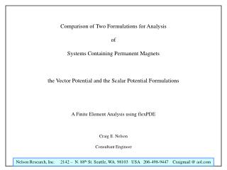
1. Comparison of Two Formulations for Analysis of Systems Containing Permanent Magnets the Vector Potential and the Scalar Potential Formulations A Finite Element Analysis using flexPDE Craig E. Nelson Consultant Engineer

2. The Nature of the Problem to be Examined: There are several useful formulation for analysis of magnetostatic problems. Each has a place where it is most efficient or, based on extent knowledge of boundary or source conditions, must be used. The most commonly used formulation utilizes the “vector potential” formulation. A less common, but sometimes useful formulation is the “scalar potential” formulation. At one point, I was curious if these two formulations gave substantially similar results. The following analysis examines this question for the case of a cylindrical shaped permanent magnet with uniform magnetization in the vertical direction

3. The Vector Potential Formulation The partial differential equation to be solved is: B = mu * H = Curl(A) Where A is the magnetic vector potential, B is the magnetic flux density, H is the magnetic field intensity and mu is the magnetic permeability of a region in space. To complete the formulation, A must be defined on the solution domain boundaries and source values for H must be defined within the domain. For very general problems containing magnetic sub domains, H is defined as: H = B/mu0 – M where M is the magnetization in magnetic regions and mu0 is the magnetic permeability of vacuum. In order to apply finite element analysis with this formulation, knowledge of the magnetization and magnetic permeability of all the solution sub domain regions as a function of B, is required. This can be problematic when the starting point for analysis happens to be knowledge of the magnetization and permeability as a function of H.

4. The Scalar Potential Formulation The partial differential equation to be solved is: div ( Hs - mu0*grad(Phi) + M ) = 0 Where Phi is the magnetic scalar potential, Hs is a source of magnetic field intensity, M is the magnetization in magnetic regions and mu0 is the magnetic permeability of vacuum. To complete the formulation, Phi must be defined on the solution domain boundaries and values for Hs and M must be defined within the domain. H is defined as: Hr = - dr(phi) Hz = - dz(phi) H = vector(Hr,Hz) where r and z are the radial and axial directions B is derived by means of: B = mu0*(H + M) In order to apply finite element analysis with this formulation, knowledge of the magnetization and magnetic permeability of all the solution sub domain regions as a function of H, is required. This can be problematic when the starting point for analysis happens to be knowledge of the magnetization and permeability as a function of B.

5. Geometry for the Finite Element Model Solution

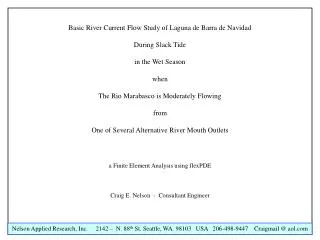
6. A and Phi = 0 A and Phi = 0 Permanent Magnet with uniform magnetization in the vertical direction Line of radial Symmetry A and Phi = 0 Solution Domain

7. A and Phi = 0 Permanent Magnet with uniform magnetization in the vertical direction A and Phi = 0 Line of radial Symmetry A and Phi = 0 Solution Domain

8. Solution Plots

9. Vector Potential Formulation – B Field Scalar Potential Formulation – B Field

10. Vector Potential Formulation – H Field Scalar Potential Formulation – H Field

11. Vector Potential Formulation - (H + M) Field Scalar Potential Formulation - (H + M) Field

12. Vector Potential Formulation – B in z direction Scalar Potential Formulation – B in z direction

13. Summary and Conclusions Two formulations for solving magnetostatic problems where permanent magnets are the source of magnetic fields have been tested with a simple cylindrical magnet problem. The numerical solution results are essentially identical The two problem formulations each have their area of applicability. The vector potential formulation, though more general than the scalar potential method, is difficult or impossible to use in those cases where the magnetization and the magnetic permeabilities are known as a function of magnetic field intensity (H). The scalar potential formulation, though somewhat limited when compared to the vector potential formulation, may be used in those cases where the magnetization and the magnetic permeabilities are known as a function of magnetic field intensity (H).