Computer Graphics Overview
This overview explores the fundamentals of color representation in displays and the drawing pipeline of computer graphics. It explains the concepts of additive and subtractive color models, color perception through the eye's structures, and the role of cones and rods in vision. The drawing pipeline is dissected into stages, from model traversal to rasterization, showing how 3D objects are rendered onto 2D displays. Key topics include RGB and CMY color components, frame buffering, clipping, lighting, and shading techniques that enhance visual output.

Computer Graphics Overview
E N D
Presentation Transcript
Computer Graphics Overview Color Displays Drawing Pipeline IAT 410
Color • Light in range 400-780 nm • Tristimulus theory allows color to be reproduced by 3 color components • Subtractive: Cyan, Magenta, Yellow CMY - Used in printing • Additive: Red, Green, Blue -- RGB IAT 410
Perception • Eye has light sensitive cells on the retina: • Cones - 3 Types • “Red”, “Green”, and Blue • Spectral Response Curves • Rods - “monochrome” IAT 410
Color Perception IAT 410
Perception • Fovea is the high-resolution area the eye • Cones are mostly at the Fovea • Cones aren’t very sensitive • Not too useful in the dark • Long temporal response time • Rods are placed all over retina • Night vision • Peripheral vision IAT 410
Additive Color • Additive: Red, Green, Blue -- RGB • Red + Blue + Green light added together = White • Basis of Color CRT 1 2 IAT 410
Displays • Color CRT contains rectangular array of colored dots - Pixels • RGB Triads • R, G, and B controlled separately per pixel • 8 bits for each R, G and B • In a 1280 x 1024 pixel display, have • 1280 x 1024 x 3 bytes per image • Refreshed 60 or more times/second: • 225 Megabytes/Sec IAT 410
Frame Buffer • Stores image to be refreshed on CRT • Dual port: Refresh port + Random-access port • Video RAM • Random-Access port used to load frame buffer with images IAT 410
Drawing Pipeline • Standard drawing process uses a pipeline of computations • Starts with: Collection of polygons • Ends with: Image stored in frame buffer (Desired result) IAT 410
Pipeline Input device -> Model traversal -> Model transform -> Viewing transform -> Clipping -> Project & Map to Viewport -> Lighting -> Shading -> Rasterization -> Display IAT 410
Pipeline:Model Traversal • Data structure of Polygons • Each polygon in own coordinate system • List: 0 1 2 3 IAT 410
y 0 1 2 3 x Pipeline: Modeling Transform • Move each polygon to its desired location • Operations: Translate, Scale, Rotate IAT 410
Clipping • Viewport is area of Frame Buffer where new image is to appear • Clipping eliminates geometry outside the viewport Resulting Polygon Clipping Viewport IAT 410
Rasterization • Find which pixels are covered by polygon: • Plane Sweep: For each polygon • go line-by-line from min to max • go from left boundary to right boundary pixel by pixel • Fill each pixel • 2D Process IAT 410
Data Representation • 2D Objects: (x, y) • 3D Objects: (x, y, z) • 2D Scale: (Sx, Sy) • 2D Rotate (R theta) • 2D Translate (Tx, Ty) ( ) ( ) Sx 0 2 0 x 4 = 8 0 Sy 0 3 4 12 IAT 410
Homogeneous coordinates • Translate(Tx, Ty, Tz) • X’ = X + Tx • Y’ = Y + Ty • Z’ = Z + Tz IAT 410
Homogeneous Coordinates • Add a 4th value to a 3D vector • (x/w, y/w, z/w) <-> (x, y, z, w) IAT 410
3D Graphics IAT 410
Project & Map to Viewport • Viewport is area of Frame Buffer where new image is to appear • Projection takes 3D data and flattens it to 2D Eye Projection Plane (Screen) IAT 410
Specular Diffuse (Lambertian) Lighting • Simulate effects of light on surface of objects • Each polygon gets some light independent of other objects IAT 410
Shading • Lighting could be calculated for each pixel, but that’s expensive • Shading is an approximation: • Gouraud shading: Light each vertex • Interpolate color across pixels IAT 410
Rendering Pipeline Input device -> Model traversal -> Model transform -> Viewing transform -> Clipping -> Project & Map to Viewport -> Lighting -> Shading -> Rasterization -> Display IAT 410