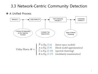
Community Detection Algorithm and Community Quality Metric
Community Detection Algorithm and Community Quality Metric. Mingming Chen & Boleslaw K. Szymanski Department of Computer Science Rensselaer Polytechnic Institute. Community Structure. Many networks display community structure

Community Detection Algorithm and Community Quality Metric
E N D
Presentation Transcript
Community Detection Algorithm and Community Quality Metric MingmingChen & Boleslaw K. Szymanski Department of Computer Science Rensselaer Polytechnic Institute
Community Structure • Many networks display community structure • Groups of nodes within which connections are denser than between them Community detection algorithms Community quality metrics
Two Related Community Detection Topics • Community detection algorithm • LabelRank: a stabilized label propagation community detection algorithm • LabelRankT: extended algorithm for dynamic networks based on LabelRank • A new community quality metric solving two problems of Modularity • M. E. J. Newman, 2006; • Newman and Girvan, 2004. Xie and Symanski, 2013. Xie, Chen, and Symanski, 2013.
LabelRank Algorithm • Four operators applied to the labels • Label propagation operator • Inflation operator • Cutoff operator • Conditional update operator No No Question: NP=P ? Node 1: No; Node 2: No; Node 3: No; Node 4: Yes. 2 3 1 1 No 1 1 97 1 P1 (No)=3/100; P1 (Yes)=97/100. P1 (No)=3/4; P1 (Yes)=1/4. Yes 4 Node 1: No. Node 1: Yes.
Label Propagation Operator • where W is the n x n weighted adjacent matrix. P is the n x n label probability distribution matrix which is composed of n (1 x n) row vectors Pi, one for each node • Each element Pi(c) holds the current estimation of probability of node i observing label , where C is the set of labels (here, suppose C={1, 2, …, n}) • Ex. Pi=(0.1, 0.2, …, 0.05, …) • To initialize P, each node is assigned a distribution of probabilities of all incoming edges
Label Propagation Operator • Each node receives the label probability distribution from its neighbors and computes the new distribution P3= (0.25, 0, 0.25, 0, 0, 0, 0.25, 0.25, 0, 0) P1= (0.25, 0.25, 0.25, 0.25, 0, 0, 0, 0, 0, 0) P1= (0.25, 0.125, 0.125, 0.125, 0.0625, 0.0625, 0.0625, 0.0625, 0.0625, 0.0625) P2= (0.25, 0.25, 0, 0, 0.25, 0.25, 0, 0, 0, 0) P4= (0.25, 0, 0, 0.25, 0, 0, 0, 0, 0.25, 0.25)
Inflation Operator • Each element Pi(c) rises to the inthpower: • It increases probabilities of labels with high probability but decreases that of labels with low probabilities during label propagation. P1= (0.25, 0.125, 0.125, 0.125, 0.0625, 0.0625, 0.0625, 0.0625, 0.0625, 0.0625) P1= (0.129, 0.0323, 0.0323, 0.0323, 0.00806, 0.00806, 0.00806, 0.00806, 0.00806, 0.00806)
Cutoff Operator • The cutoff operator on P removes labels that are below the threshold with the help from Inflation Operator that decreases probabilities of labels with low probabilities during propagation. • efficiently reduces the space complexity from quadratic to linear. P1= (0.129, 0.0323, 0.0323, 0.0323, 0.00806, 0.00806, 0.00806, 0.00806, 0.00806, 0.00806) With r = 0.1, the average number of labels in each node is less than 3. P1= (0.129)
Conditional Update Operator • At each iteration, it updates a node i only when it is significantly different from its incoming neighbors in terms of labels: • where is the set of maximum probability labels at node i at the last step. returns 1 if and 0 otherwise. ki is the node degree and q∈[0,1]. • isSubset can be viewed as a measure of similarity between two nodes.
Running time of LabelRank • O(Tm): m is the number of edges and T is the number of iterations. LabelRank is a linear algorithm
LabelRankT • It is a LabelRank with one extra conditional update rule by which only nodes involved changes will be updated. Changes are handled by comparing neighbors of node i at two consecutive steps, and .
Two Problems of Modularity Maximization • Split large communities • Favor small communities • Resolution limit problem • Modularity optimization may fail to discover communities smaller than a scale even in cases where communities are unambiguously defined. • This scale depends on the total number of edges in the network and the degree of interconnectedness of the communities. • Favor large communities Fortunato et al, 2008; Li et al, 2008; Arenas et al, 2008; Berry et al, 2009; Good et al, 2010; Ronhovde et al, 2010; Fortunato, 2010; Lancichinetti et al, 2011; Traag et al, 2011; Darst et al, 2013.
Modularity • Modularity (Q): the fraction of edges falling within communities minus the expected value in an equivalent network with edges placed at random • Equivalent definition M. E. J. Newman, 2006. Newman and Girvan, 2004.
Modularity with Split Penalty • Modularity (Q): the modularity of the community detection result • Split penalty (SP): the fraction of edges that connect nodes of different communities • Qs= Q – SP: solving the problem, favoring small communities, of Modularity
Qs with Community Density • Resolution limit: Modularity optimization may fail to detect communities smaller than a scale • Intuitively, put density into Modularity and Split Penalty to solve the resolution limit problem • Equivalent definition
Example of One Complete Graph Community Quality on a complete graph with 8 nodes
5-clique Example ∆Qs=(0.8424-0.7848)=0.0576 > ∆Q=(0.8879-0.8758)=0.0121
Thanks! Q & A