Download
1 / 31
360 likes | 820 Vues
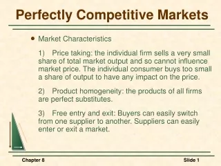
Perfectly Competitive Markets. Market Characteristics 1) Price taking: the individual firm sells a very small share of total market output and so cannot influence market price. The individual consumer buys too small a share of output to have any impact on the price.

E N D
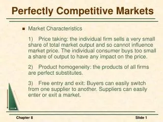
Perfectly Competitive Markets • Market Characteristics 1) Price taking: the individual firm sells a very small share of total market output and so cannot influence market price. The individual consumer buys too small a share of output to have any impact on the price. 2) Product homogeneity: the products of all firms are perfect substitutes. 3) Free entry and exit: Buyers can easily switch from one supplier to another. Suppliers can easily enter or exit a market. Chapter 8
Profit Maximization • Do firms maximize profits? • Possibility of other objectives • Revenue maximization • Dividend maximization • Short-run profit maximization • Implications of non-profit objective • Over the long-run investors would not support the company • Without profits, survival unlikely Chapter 8
Marginal Revenue, Marginal Cost and π Maximization • Determining the profit maximizing level of output • Profit ( ) = Total Revenue - Total Cost • Total Revenue (R) = Pq • Total Cost (C) = Cq • Therefore: Chapter 8
Total Revenue R(q) Slope of R(q) = MR Profit Maximization in the Short Run Cost, Revenue, Profit ($s per year) 0 Output (units per year) Chapter 8
C(q) Total Cost Slope of C(q) = MC Why is cost positive when q is zero? Profit Maximization in the Short Run Cost, Revenue, Profit $ (per year) 0 Output (units per year) Chapter 8
C(q) R(q) A B q0 q* Marginal Revenue, Marginal Cost and π Maximization • Comparing R(q) and C(q) • Output levels: 0 - q0: • C(q)> R(q): negative profit • FC + VC > R(q) • MR > MC • Output levels: q0 - q* • R(q)> C(q) • MR > MC: higher profit at higher output. Profit is increasing Cost, Revenue, Profit ($s per year) 0 Output (units per year) Chapter 8
Cost, Revenue, Profit $ (per year) C(q) R(q) A B q0 q* 0 Output (units per year) Marginal Revenue, Marginal Cost and π Maximization • Comparing R(q) and C(q) • Output level: q* • R(q)= C(q) • MR = MC • Profit is maximized Chapter 8
$4 d $4 D Demand and MR Faced by a Competitive Firm Price $ per bushel Price $ per bushel Firm Industry Output (millions of bushels) Output (bushels) 100 200 100
Marginal Revenue, Marginal Cost and π Maximization • The competitive firm’s demand • Individual firm sells all units for $4 regardless of their level of output. • If the firm tries to raise price, sales are zero. • If the firm tries to lower price, he cannot increase sales • P = D = MR = AR • Profit Maximization: MC(q) = MR = P Chapter 8
MC Lost profit for q1 < q* Lost profit for q2 > q* A D AR=MR=P ATC C B AVC At q*: MR = MC and P > ATC q1 : MR > MC and q2: MC > MR and q0: MC = MR but MC falling q0 q1 q* q2 A Competitive Firm making a Positive Profit: SR Price ($ per unit) 60 50 40 30 20 10 0 1 2 3 4 5 6 7 8 9 10 11 Output Chapter 8
MC ATC B C D P = MR A At q*: MR = MC and P < ATC Losses = (P- AC) q* or ABCD AVC F E q* A Competitive Firm Incurring Losses: SR Price ($ per unit) Would this producer continue to produce with a loss? Output Chapter 8
Choosing Output in the Short Run • Summary of Production Decisions • Profit is maximized when MC = MR • If P > ATC the firm is making profits. • If AVC < P < ATC the firm should produce at a loss. • If P < AVC < ATC the firm should shut-down. Chapter 8
The firm chooses the output level where MR = MC, as long as the firm is able to cover its variable cost of production. MC ATC P2 AVC P1 What happens if P < AVC? P = AVC q1 q2 A Competitive Firm’s Short-Run Supply Curve Price ($ per unit) Output Chapter 8
A Competitive Firm’s Short-Run Supply Curve S = MC above AVC Price ($ per unit) MC ATC P2 AVC P1 P = AVC Shut-down Output q1 q2 Chapter 8
Input cost increases and MC shifts to MC2 and q falls to q2. MC2 Savings to the firm from reducing output MC1 $5 q2 q1 The Response of a Firm to a Change in Input Price Price ($ per unit) Output Chapter 8
S The short-run industry supply curve is the horizontal summation of the supply curves of the firms. MC1 MC2 MC3 P3 P2 P1 Industry Supply in the Short Run $ per unit Question: If increasing output raises input costs, what impact would it have on market supply? Quantity 0 2 4 5 7 8 10 15 21 Chapter 8
The Short-Run Market Supply Curve • Elasticity of Market Supply • Perfectly inelastic short-run supply arises when the industry’s plant and equipment are so fully utilized that new plants must be built to achieve greater output. • Perfectly elastic short-run supply arises when marginal costs are constant. Chapter 8
At q* MC = MR. Between 0 and q , MR > MC for all units. Producer Surplus MC AVC B A P Alternatively, VC is the sum of MC or ODCq* . R is P x q*or OABq*. Producer surplus = R - VC or ABCD. D C q* Producer Surplus for a Firm Price ($ per unit of output) 0 Output Chapter 8
The Short-Run Market Supply Curve • Producer Surplus in the Short-Run Chapter 8
S Market producer surplus is the difference between P* and S from 0 to Q*. P* Producer Surplus D Q* Producer Surplus for a Market Price ($ per unit of output) Output Chapter 8
In the long run, the plant size will be increased and output increased to q3. Long-run profit, EFGD > short run profit ABCD. LMC LAC SMC SAC D A E $40 P = MR C B G F $30 In the short run, the firm is faced with fixed inputs. P = $40 > ATC. Profit is equal to ABCD. q1 q2 q3 Output Choice in the Long Run Price ($ per unit of output) Output Chapter 8
LMC LAC SMC SAC E $40 P = MR $30 Output Choice in the Long Run Price ($ per unit of output) Question: Is the producer making a profit after increased output lowers the price to $30? D A C B G F q1 q2 q3 Output Chapter 8
Choosing Output in the Long Run Long-Run Competitive Equilibrium • Zero-Profit • If R > wL + rK, economic profits are positive • If R = wL + rK, zero economic profits, but the firm is earning a normal rate of return; indicating the industry is competitive • If R < wL + rK, consider going out of business Chapter 8
Profit attracts firms • Supply increases until profit = 0 S1 LMC P1 LAC S2 $30 P2 D Q1 Q2 Long-Run Competitive Equilibrium $ per unit of output $ per unit of output Firm Industry $40 q2 Output Output
Choosing Output in the Long Run • Long-Run Competitive Equilibrium 1) MC = MR 2) P = LAC • No incentive to leave or enter • Profit = 0 3) Equilibrium Market Price Chapter 8
Choosing Output in the Long Run • Questions 1) Explain the market adjustment when P < LAC and firms have identical costs. 2) Explain the market adjustment when firms have different costs. 3) What is the opportunity cost of land? Chapter 8
Choosing Output in the Long Run • Economic Rent = the difference between what firms are willing to pay for an input minus the minimum amount necessary to obtain it. • An Example: Two firms, A & B, both own their land • A is located on a river which lowers A’s shipping cost by $10,000 compared to B. The demand for A’s river location will increase the price of A’s land to $10,000 • Economic rent = $10,000 • $10,000 - zero cost for the land • Economic rent increases; Economic profit of A = 0 Chapter 8
The Industry’s Long-Run Supply Curve • The shape of the long-run supply curve depends on the extent to which changes in industry output affect the prices the firms must pay for inputs. • To determine long-run supply, we assume: • All firms have access to the available production technology. • Output is increased by using more inputs, not by invention. • The market for inputs does not change with expansions and contractions of the industry. Chapter 8
Economic profits attract new firms. Supply increases to S2 and the market returns to long-run equilibrium. Q1 increase to Q2. Long-run supply = SL = LRAC. Change in output has no impact on input cost. S1 S2 MC AC C P2 P2 A B SL P1 P1 D1 D2 q1 q2 Q1 Q2 LR Supply in a Constant-Cost Industry $ per unit of output $ per unit of output Output Output
Due to the increase in input prices, long-run equilibrium occurs at a higher price. S1 S2 LAC2 SMC2 SL SMC1 P2 LAC1 P2 P3 P3 B A P1 P1 D1 D1 q1 q2 Q1 Q2 Q3 LR Supply in an Increasing-Cost Industry $ per unit of output $ per unit of output Output Output
Due to the decrease in input prices, long-run equilibrium occurs at a lower price. S1 S2 SMC1 LAC1 SMC2 P2 P2 LAC2 P1 A P1 B P3 P3 SL D1 D2 q1 q2 Q1 Q2 Q3 LR Supply in a Decreasing-Cost Industry $ per unit of output $ per unit of output Output Output