
EM Algorithm for Genotype-Phenotype Association in Mouse Strains
Explore a model relating genotype and phenotype in mice using EM algorithm, estimating parameters and testing for associations. Implementations in R and Matlab included for easy application.

EM Algorithm for Genotype-Phenotype Association in Mouse Strains
E N D
Presentation Transcript
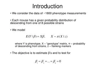
Introduction We consider the data of ~1800 phenotype measurements Each mouse has a given probability distribution of descending from one of 8 possible strains We model where Y is phenotype, X – “genotype” matrix, π – probability of descending from strains, z – flanking markers The objective is to estimate β’s and to test for
Approaches Linear regression replace the true design matrix with E(X) and the estimator is given by - estimator is unbiased - normally distributed - linear in Y - has large variance due to collinearity
Approaches (2) Maximum likelihood estimator Maximize with respect to β: - expression simplifies - easy to evaluate point-wise - functional form not known, hence difficult to optimize - properties of the MLE are unknown
Approaches (3)Use a stochastic optimiser for finding MLE: the EM The two steps are: E-step, calculate for i-th mouse (only for categorical covariates) M-step, maximize Q w.r.t. β Advantages: Automatic Fast Approximate distribution of estimates allows to perform testing Easily generalised to GLM
Implementation of the EM M-step becomes equivalent to a Weighted Least Squares or a weighted GLM model (fitting routines available in R and Matlab): Where Y and X are augmented matrices, the weights matrix constructed using HMM output. Below there are only results for normal distribution of Y but the EM was applied to the binomial and exponential cases as well.
Augmenting the model Given the phenotypes Y and the weights W we create the model: with corresponding weights
Simulated example: generated phenotypes Response generated for set variance 0.3 and β = (1,0,0,0,0,0,0,0)
Running the EM Values of β parameters at the EM iterations. The real values are (1,0,0,0,0,0,0,0).
Running time 10 seconds - approximate running time for the WLS case - on 1,649 mice - implemented in Matlab - with convergence achieved at 15 iterations for some starting points 60 seconds - For 3,298 mice
Testing Likelihood ratio test performed for the EM linear regression with known design matrix linear regression with the expectation of design matrix. under collinearity
Empirical null distributions • EM algorithm null distribution E(X) case null distribution
Power curves Description of the power of the LR test All β’s set to 0 except first one Simulate data sets and plot number of rejections For each value of β 500 simulations were performed
Simulated power curves Randomly drawn combination of progenitor strains Least likely combination of progenitor strains Most likely combination of progenitor strains
Data Considered OpenArmTime phenotype ~200 mice have zero records and were removed Is it a mixture of normal distributions?
Future development Time to event models - Censored data - Cox proportional hazards model Bayesian models Implementation in R Models for multivariate phenotypes Multiple hypothesis testing HMM improvement


