Download
1 / 31
310 likes | 397 Vues
Explore the significance of non-Gaussian perturbations in the CMB bispectrum and their implications for cosmological models. Investigate the impact of nonlinearities on observational data and the need for accurate computational models.

E N D
Quantifying nonlinear contributionsto the CMB bispectrumin Synchronous gauge Guido W. Pettinari Institute of Cosmology and Gravitation University of Portsmouth Under the supervision of Robert Crittenden YITP, CPCMB Workshop, Kyoto, 21/03/2011
Outline • Why non-Gaussianities? • Why go to 2nd order? • Why do it in Synchronous gauge? • Some details & first results
Gaussian perturbations • At 1st perturbative order, the CMB anisotropies take over the non-Gaussianity, if any, from the primordial fluctuations • ... which implies that the CMB angular bispectrum vanishes for Gaussian primordial perturbations • ... thus leading to a nice Gaussian CMB map for simple inflationary scenarios:
Gaussian perturbations • ~ 1 million pixels
Gaussian perturbations • ~ 1 thousand numbers
Non-Gaussianities • Many models of the early Universe produce non-Gaussian perturbations. Here is a very incomplete list: Linde & Mukhanov, 1997 Lyth, Ungarelli & Wands, 2003 • Curvaton scenario Bernardeau & Uzan, 2002, 2003 Lyth & Rodriguez, 2005, Naruko & Sasaki, 2009 • Multi-scalar field inflaton models • DBI inflation Alishahiha, Silverstein & Tong 2004 Chambers & Rajantie, 2008 Enqvist & al., 2005 • Inflationary models with pre-heating Khoury, Ovrut, et al., 2001 Steinhardt & Turok, 2002 • Ekpyrotic universe • These models produce quite different non-Gaussian distributions. We shall focus on those that admit a simple local parametrisation: Quadratic correction
Non-Gaussianities • Measurements so far are consistent with Gaussianity, but still leave room for some non-Gaussianities: Komatsu et al., AJS (2011) Slosar et al., JCAP (2008) • The upcoming PLANCK experiment promises to reduce the error bars by a factor 4, down to WMAP7 : PLANCK : • fNL is very difficult to measure! SDSS :
The effect is very small • Unnoticeable by eye unless fNL > 1000 Liguori, Sefusatti, Fergusson, Shellard, 2010
The effect is very small • Gaussian realization of a CMB temperature map Liguori, Sefusatti, Fergusson, Shellard, 2010
The effect is very small • Gaussian realization with a local fNL= 3000 superimposition Liguori, Sefusatti, Fergusson, Shellard, 2010
Non-Linearities • Any non-linearities can make initially Gaussian perturbations non-Gaussian e.g. Komatsu, CQG, 2010 Liguori et al., AiA 2010 • Galactic foregrounds • Unresolved point sources • etc ... • Lensing – ISW correlation • Detector-induced noise We shall focus on how non-linearities in Einstein equations affect the CMB bispectrum by going to second perturbative order
Non-Linearities Term quadratic in the primordial fluctuations e.g. Komatsu, CQG, 2010 Nitta et al., 2009 Second-order transfer function The initial conditions are propagated nonlinearly into the observed CMB anisotropies
Non-Linearities • Both primordial & late time evolution can generate NG. In particular: • Above linear order, it is not true that Gaussian initial conditions imply Gaussianity of the CMB • The shape of the second order bispectrum is determined by the shape of the second-order radiation transfer function • Example: If • then, even with primordial NG of the local type, • the contribution to fNL would be small It is crucial to predict the shape and amplitude of second-order effects, in order to subtract them from the data
Previous results • So far, the only full numerical calculation of F (2) was made in Newtonian gauge: • Pitrou, Uzan & Bernardeau, JCAP, 2010
Previous results • So far, the only full numerical calculation of F (2) was made in Newtonian gauge: • N.B. For a treatment of only the quadratic terms, please refer to Nitta, Komatsu, Bartolo, Matarrese, Riotto, 2009
Previous results • Some details on the numerical computation by Pitrou et al.: • They adopt Newtonian gauge • The code, CMBQuick, is made with Mathematica and it is publicly available • Non-parallel code, it takes two weeks to calculate the full bispectrum
Our purpose • The result by Pitrou et al. implies that late-time non-Gaussianities are important, and lay right on Planck’s detection threshold • If the result is confirmed, the CMB maps from Planck and other experiments need to be cleaned of these second-order effects via the construction of templates Komatsu, CQG, 2010 • It is therefore crucial to double-check the computation by Pitrou et al, possibly in an independent way
Our purpose • In collaboration with Cyril Pitrou, we aim to confirm and improve the above mentioned results by: • Writing from scratch a low-level 2nd order Boltzmann code to derive the full radiation transfer function • Performing the calculations in Synchronous gauge • Making the code parallel, object-oriented and flexible, in order to allow easy customizations (e.g. add another gauge or model) • Using open-source libraries (GSL, Blas, Lapack...)
Why Synchronous gauge? • Difficult to have the same errors using different gauges • Synchronous gauge is more apt to numerical solving • e.g. COSMICS, CMBFast, CAMB, CMBEasy • Comparing results of two different gauges may help detect possible gauge artifacts • Nobody has done it yet
Structure of the code-to-be • Two main components: • Mathematica package to derive the equations • powerful symbolic algebra system • C++ code to solve them numerically • fast, supports object oriented programming • Both can be used independently, but will be able to communicate • Input the (long!) equations to be solved numerically from within Mathematica • Example:
Structure of the code-to-be • The Mathematica package is (almost) complete, and includes original sub-packages designed to perform: • Tensor manipulation • allows for natural input of tensor operations • Metric Perturbations • derive geometrical quantities in any gauge, at any order • Fourier transformation of equations • e.g. accounts for convolutions arising from non-linear terms • Collection of terms • spot terms such as
A taste of 2nd order PT • Continuity equation in Synchronous gauge (only scalar DOF) • 76terms, and it is one of the simplest equations
A taste of 2nd order PT • Fourier space + term collection... • Similarly, we derived Einstein & Euler equations, and checked them against Tomita (1967) • We also found equations in Newtonian gauge, and checked them against Pitrou et al. (2008, 2010)
Conclusions • We need to adopt a 2nd order perturbative approach to quantify contamination to primordial fNL from late non-linear evolution • The full second order transfer function F(2) is needed to properly subtract the effect (non-trivial!!!) • Synchronous gauge is suitable to perform the computation, and will lead to an independent confirmation of Pitrou et al. results (fNL ~ 5 for both squeezed and equilateral shapes) • We already derived most relevant equations, and will integrate them numerically by means of a parallel, object-oriented, low-level code
Lensing-ISW correlation Komatsu, CQG, 2010
Synchronous scalar perturbations • Metric perturbations at second order • Energy-momentum tensor perturbations at second order (space part)
Synchronous gauge fixing 1 Malik & Wands, 2009
Synchronous gauge fixing 2 Malik & Wands, 2009 M. Bucher, K. Moodley, N. Turok, Phys. Rev. D 62 (2000)