Linear Functional Fixed-Points
This overview discusses linear functional fixed-point (FFP) logic, exploring complexity results and integrations with SMT solvers like Z3. It investigates the complexity of various forms of FFP, including propositional, linear, and non-linear cases, providing insights into their PSPACE and NEXPTIME hardness. The document also outlines practical reasoning approaches, the role of quantifier-free theories, and encoding challenges in fixed-point logic. It emphasizes the significance of combining sequential decision procedures for effective automation in reasoning about program verification and other applications. ###

Linear Functional Fixed-Points
E N D
Presentation Transcript
Linear Functional Fixed-Points Nikolaj Bjørner Joe Hendrix Microsoft Research & Corporation
Overview • Linear Functional Fixed-Point Logic (FFP) • Complexity results for FFP: • FFP(Propositional) – PSPACE/NP • FFP(Linear/Equalities) – PSPACE • By a reduction to LTL • FFP(Non-linear)– NEXPTIME hard/undecidable • Integrating FFP with an SMT solver (Z3)
A list-manipulating program head head head curr curr := head T T F F T T F F data(curr) := true; curr := f(curr) F T F T F F T F T F T F F F F T curr curr curr head curr = head Loop invariant: Every data element between head and curr is set to true
The loop invariant head Loop invariant: Every data element between head and curr is set to true F T f x [head curr] . data(x) T F T F invariant(head) where invariant(x) = x = curr (data(x) invariant(f(x))) curr LFP Inv , x. [ x = curr (data(x) Inv(f(x))) ] (head) Inv x [ x = curr (data(x) Inv(f(x))) ] (head) What are practical ways of reasoning with such fixed-points?
Some solutions f f w u v f f f f f uv w [Nelson 80]
Some solutions w u v f f f f f f f uv btwnf(u,v,w) [Rakamarić07+] w [Nelson 80]
Some solutions BSet(f(f(u))) BSet(u) From u reach vand v is the first element satisfyingBSet(v) B(u) = v u v f f f f BSet(v) BSet(f(u)) BSet(f(f(u))) From u reach vand everything afteru and up to v satisfies BSet u v R(u,v) f f f f BSet(f(u)) f uv wf. Reachability [Lahiri, Qadeer 06] btwnf(u,v,w) • [Rakamarić07+] w [Nelson 80]
Some solutions Use first-order axioms to encode quantifier-free theory of reachability. [LQ08] rely on SMT solver Z3 for instantiating axioms using triggers. Required quantifier support by solver is not so off-the-shelf. Interpreted sets & Bounded quant. [Lahiri, Qadeer 08] f uv wf. Reachability [Lahiri, Qadeer 06] btwnf(u,v,w) • [Rakamarić07+] w [Nelson 80]
Some solutions SnS (inf.Trees) SO(f) (infinite trees) S1S (inf. Acyclic lists) wSnS (finite trees) wSO(f) (finite linked lists) wS1S (fin. Acyclic lists) FFP(Non-linear) Reachable Patterns [Yorsh+ 06] Lin. FFP(Eq) Interpreted sets & Bounded quant. [Lahiri, Qadeer 08] FFP(Prop) f uv wf. Reachability [Lahiri, Qadeer 06] btwnf(u,v,w) • [Rakamarić07+] w [Nelson 80]
Many other solutions • [Immerman+ 04] First-order transitive closure • [Møller+ 05] Pointer assertion logic • [Lev-Ami+ 05] Acyclic transtive closure • [McPeak+ 05] Linked lists • [Ranise+ 05] Linked lists • [Balaban+ 07] Single parent heaps • [Bouajjani+ 06-09] Reachability + arithmetic + T • Apologies for relevant omissions.
A Quest for an SMT solver integration • Existing decision procedures for fixed-points use • Encoding with first-order axioms • Rely on first-order instantiation engine for completeness • Reduction to automata • Powerful combination with some theories, but flexible combination approach and “low-order” complexity results unclear to us head F T T F T F curr
The DPLL(T) setting for SMT Specialized theory solvers interoperate by exchanging learned equalities and clauses with a common congruence closure core Theories Formula head Bit-Vectors T F Rewriting Simplification Arithmetic F T T F curr Core Theory Arrays E-matching Data-types SAT solver Core Theory: Equalities, asserted literals Theory Core: Equalities, asserted literals, new clauses
Back to the loop invariant Loop invariant: Every data element between head and curr is set to true head F T f x [head curr] . data(x) T F T F invariant(head) where invariant(x) = x = curr (data(x) invariant(f(x))) curr LFP Inv , x. [ x = curr (data(x) Inv(f(x))) ] (head) Inv x [ x = curr (data(x) Inv(f(x))) ] (head)
Question: Is there a convenient propositional-likeabstraction of fixed-points? Our Approach: establish and use a connection with Linear Time Temporal Logic for linear functional fixed-points head T F F T T F curr A Until B [data(x) Untilf,xx = curr] (head) B [A (A Until B)] X . B [A X] Inv x [ x = curr (data(x) Inv(f(x))) ] (head)
FFP Temporal Macros • [A(x) Untilf,xB(x)] (a) R x [B(x) (A(x) R(f(x)))] (a) • [f,xA(x)] (a) [trueUntilf,xA(x)] (a) • [f,xA(x)] (a) [f,xA(x)] (a)
Some solutions SnS (inf.Trees) SO(f) (infinite trees) S1S (inf. Acyclic lists) wSnS (finite trees) wSO(f) (finite linked lists) wS1S (fin. Acyclic lists) FFP(Non-linear) Reachable Patterns [Yorsh+ 06] Lin. FFP(Eq) Interpreted sets & Bounded quant. [Lahiri, Qadeer 08] FFP(Prop) f uv wf. Reachability [Lahiri, Qadeer 06] btwnf(u,v,w) [Rakamanic07+] w [Nelson 80]
Our approach – a tighter sandwich Propositional Linear Time Temporal Logic ? FFP(Non-linear) Reachable Patterns [Yorsh+ 06] Lin. FFP(Eq) Interpreted sets & Bounded quant. [Lahiri, Qadeer 08] FFP(Prop) f uv wf. Reachability [Lahiri, Qadeer 06] btwnf(u,v,w) [Rakamanic07+] w [Nelson 80]
FFP(Propositional Logic): basic results [f,xP(f(x))](a) [f,xP(x)](b) [Q(x) Untilf,xP(f(x))](b) - Distinguished function f - Unary predicate symbols, P, Q, R - At most one bound variable in scope at any time [Q(x) Untilf,x[P(f(x)) Untilf,yR(y)]](b)
FFP(PL): basic results • From LTL to FFP(PL) P f,xf,xP(f(x))(anchor) • From FFP(PL) to LTL f,xP(f(x))(a) f,xP(x)(b) Pa Pb • Complexity(FFP(PL)) = Complexity(pLTL)
FFP(Equalities): propositions and equalities f f u v u v f f f f [True Untilf,xx = v](u) f,x(x = v)(u)
FFP(E): propositions and equalities f f f u v w w u v f f f f [x w Untilf,xx = v](u)
FFP(E): propositions and equalities w u v btwnf(u,v,w) f f f f f f [x w Untilf,xx = v](u) f,x(x = w)(v)
FFP(E): propositions and equalities BSet(f(f(u))) BSet(u) B(u) = v u v f f f f BSet(v) BSet(f(u)) [BSet(x) Untilf,xx = v](u) BSet(v) BSet(f(f(u))) u v R(u,v) f f f f BSet(f(u)) [BSet(f(x)) Untilf,xx = v](u)
FFP(E): propositions and equalities [f,xx c](b) [g,xP(g(x))](a) [f,xP(f(x))](a) [x fff(x) Untilf,xx = a](b) [g,xg(g(x)) = x](c) • Distinguished functions f, g • As long as f and g are separate • Unary predicate symbols, P, Q, R • At most one bound variable in scope at any time
FFP(E): A litmus test. Closure under updates. wp(f(u) := v, [A Untilf,xB](w)) f’ := x. if x = u then v else f(x) = [AUntilf,xB](w)[f f’] A’ := A[f f’], B’ := B[f f’] = [A’ Untilf’,xB’](w) = …. = [A’’ Untilf,xB’’](w) A’’ := A’ u xB’’ := B’ (u = x [(u x A’) Untilf,xB’](v))
FFP(E) : reduction to LTL? • From LTL to FFP(E) P f,xf,xP(f(x))(anchor) • From FFP(E) to LTL? [f,xx = c f,xP(x)](a) a and b reach c [f,xx = c f,xP(x)](b) after that there is a commonPstate.
FFP(E) : reduction to LTL? • From LTL to FFP(E) P f,xf,xP(f(x))(anchor) • From FFP(E) to LTL [f,x(T(x) U(x)) f(x) = b](a) [f,x(T(x) U(x)) f(x) = c](b) [f,x(T(x) U(x)) f(x) = a](c) a c T U U T Obstacle: f is a function.- The Temporal Next operator does not encode functionality by itself. U b T
FFP(E) encoding forcing functionality Normalize Functionality axioms f Erasure PTL Tableau() F – acc. cond PTL* Functionality axioms
FFP(E) encoding forcing functionality Normalize Functionality axioms f Erasure PTL Tableau() F – acc. cond PTL* Pure pLTL formula Proposition: Validity for FFP(E) is PSPACE complete Size of PTL* is quadratic in
FFP(E) extensions FFP(NL) – more than one variable in nested bound context [f,x[f,yf(x) y](x)] (a) NEXPTIME hard FFP(NL) MSO(f) 2FFP(E) – allow nested use of functions f g: [f,xg(f(x)) = f(g(x))] (a) 2FFP(E) is undecidable a f f f f f f f a f f f f f f g g g g g g f f f f f f g g g g g g
SMT solver Integration • Most SMT solvers use a DPLL(T) architecture SAT Equality Core Theories SAT Equality Core Theories Literal assignments Equalities Literal assignments Literal assignments Equalities Literal assignments Lemmas (Conflict Clauses)
SMT solver Integration (Theory) • Property: FFP(E) is stably infinite • If FFP(E) formula has a model, it has a model of size N, it has a model of size N+1 • Theorem: Let T be stably infinite, decidable, and have disjoint signature from f, g, Then quantifier-free formulas over FFP(E) + Tare decidable
SMT solver Integration (Incremental) pLTLEquality Core Theories pLTLEquality Core Theories Equalities Literal assignments Trace of Literal assignments Equalities Literal assignments Invariants Safety properties
Summary • Linear Functional Fixed-Point Logic (FFP) • Complexity results for FFP: • FFP(Propositional) – PSPACE/NP • FFP(Linear/Equalities) – PSPACE • By a reduction to LTL • FFP(Non-linear)– NEXPTIME hard/undecidable • Integrating FFP with the SMT solver
Conclusions • We established a sandwich link between • Linear Functional Fixed-Point Logic and • Propositional Linear Time Temporal Logic • More sandwiched links plausible, but open. • From DPLL(T) to SMC(T) • We show how to integrate a solver based on LTL with an SMT Solver • A prototype using CUDD and shows signs of life