Intercomparison of Drift Floats in an Intermediate Current Regime
Discussing sources of underwater speed "contamination" and suggesting improvements for underwater velocity measurements. Presenting results of float drift data versus known lagrangian references for improving accuracy. Collaborative research between IfM Kiel and BSH Hamburg on current flow paths and velocity estimations.

Intercomparison of Drift Floats in an Intermediate Current Regime
E N D
Presentation Transcript
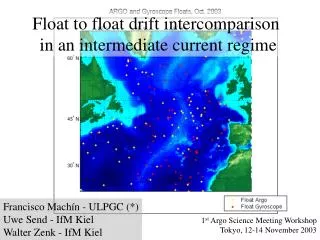
Float to float drift intercomparison in an intermediate current regime Francisco Machín - ULPGC (*) Uwe Send - IfM Kiel Walter Zenk - IfM Kiel 1st Argo Science Meeting Workshop Tokyo, 12-14 November 2003
Motivation Cycling floats 1. Hydrographic data (Wong, 2001) 2. Current fields (Davis, 1998; Schmidt, 2001) Goal: discuss sources of underwater speed “contamination” and suggest improvements underwater velocity. Raw drift data vs. known lagrangian references (APEX float) (4 RAFOS floats)
Experimental Site Observations: cooperation between the IfM Kiel and the Federal Maritime and Hydrographic Agency (BSH, Hamburg) Meteor 45 Historical Setting Paillet et al. (1998)
Experimental Site: flow paths (Zenk et al., 2000)
Experimental Site: flow paths Apex: 1500 dbar
Experimental Site: APEX cycle 1. Surface drift extrapolation a) Estimate surfacing and begin-of-descent times - Message number, - Message block number, - Repetition rate, - Times corresponding to the first and last fixes. Accuracy: 1 s
Experimental Site: APEX cycle 1. Surface drift extrapolation b) Estimate corresponding locations - cubic smooth spline fit Surfacing and begin-of-descent times too long => UW abolished
Experimental Site: APEX cycle 1. Surface drift extrapolation c) Estimate uncertainty surface mean speed: 46.4 cm s-1 mean time to extrapolate : 2.3 h Uncertainty O(3 km)
Experimental Site: APEX cycle 1. Surface drift extrapolation 2. Ascending and descending times - ascending float rate (wf): 8 cm s-1 - mission depth: 1500 m Ascending time = 5.21 h Descending time = 6 h (Webb, 2002)
Experimental Site: APEX cycle - a closer look wf= 8.5 ± 1 cm s-1
Experimental Site: APEX cycle 1. Surface drift extrapolation 2. Ascending and descending times 3. Geostrophic and Ekman shear considerations a) Geostrophic calculations - assuming synopticity between two successive profiles - lnm at deepest level (1500 m) rms geostrophic velocity was obtained Geostrophic displacement = 753 ± 927 m
Experimental Site: APEX cycle 1. Surface drift extrapolation 2. Ascending and descending times 3. Geostrophic and Ekman shear considerations b) Ekman consideration - mean wind speed: 12-16 m s-1 (NOAA) - Ekman spiral velocity, vEk - sEk, displacement by wind stress O(100 m) Uncertainties relative importance Surface drift : Geostrophic : Ekman 78 : 20 : 2
Experimental Site: Velocity comparison Background, at least: - two instruments - ten float days
Experimental Site: Initial and long-term separations a) long-term separation
Experimental Site: Initial and long-term separations b) initial separation
Experimental Site: Initial and long-term separations b) initial separation
Experimental Site: Initial and long-term separations b) initial separation - integral time scale: 8-10 d (Lankhorst, 2002) - mean advection estimate: 4 cm s-1 spatial scale = 28-36 km
Conclusions 1. In a statistical sense underwater velocities are coherent with velocities from the RAFOS reference. 2. Results are coherent with previous estimates from MARVOR floats ( Speer et al . 1999). 3. Geostrophic and wind-induced displacements are a secondary source of uncertainty. 4. Both float types trace the DWBC. 5. RAFOS floats resolve the eddy field, APEX float meanders. 6. More cases are needed to establish a more general procedure to estimate the UW drift.