Applications of Dynamic Programming

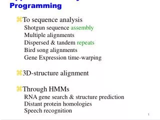
1. Applications of Dynamic Programming • To sequence analysis Shotgun sequence assembly Multiple alignments Dispersed & tandem repeats Bird song alignments Gene Expression time-warping • 3D-structure alignment • Through HMMs RNA gene search & structure prediction Distant protein homologies Speech recognition

2. Alignments & Scores Local (motif) ACCACACA :::: ACACCATA Score= 4(+1) = 4 Global (e.g. haplotype) ACCACACA ::xx::x: ACACCATA Score= 5(+1) + 3(-1) = 2 Suffix (shotgun assembly) ACCACACA ::: ACACCATA Score= 3(+1) =3

3. Increasingly complex (accurate) searches Exact (StringSearch) CGCG Regular expression (PrositeSearch) CGN{0-9}CG = CGAACG Substitution matrix (BlastN) CGCG ~= CACG Profile matrix (PSI-blast) CGc(g/a) ~ = CACG Gaps (Gap-Blast) CGCG ~= CGAACG Dynamic Programming (NW, SM) CGCG ~= CAGACG Hidden Markov Models (HMMER)

4. "Hardness" of (multi-) sequence alignment Align 2 sequences of length N allowing gaps. ACCAC-ACA ACCACACA ::x::x:x: :xxxxxx: AC-ACCATA , A-----CACCATA , etc. 2N gap positions, gap lengths of 0 to N each: A naïve algorithm might scale by O(N2N). For N= 3x109this is rather large. Now, what about k>2 sequences? or rearrangements other than gaps?

5. Testing search & classification algorithms Separate Training set and Testing sets Need databases of non-redundant sets. Need evaluation criteria (programs) Sensistivity and Specificity (false negatives & positives) sensitivity (true_predicted/true) specificity (true_predicted/all_predicted) Where do training sets come from? More expensive experiments: crystallography, genetics, biochemistry

6. Comparisons of homology scores Pearson WR Protein Sci 1995 Jun;4(6):1145-60 Comparison of methods for searching protein sequence databases. Methods Enzymol 1996;266:227-58 Effective protein sequence comparison. Algorithm: FASTA, Blastp, Blitz Substitution matrix:PAM120, PAM250, BLOSUM50, BLOSUM62 Database: PIR, SWISS-PROT, GenPept Switch to protein searches when possible

7. A Multiple Alignment of Immunoglobulins

8. Scoring matrix based on large set of distantly related blocks: Blosum62

9. Scoring Functions and Alignments • Scoring function: (match) = +1; (mismatch) = -1; (indel) = -2; (other) = 0. • Alignment score: sum of columns. • Optimal alignment: maximum score. } substitution matrix

10. Calculating Alignment Scores

11. DNA2: Aligning ancient diversity Comparing types of alignments & algorithms Dynamic programming Multi-sequence alignment Space-time-accuracy tradeoffs Finding genes -- motif profiles Hidden Markov Model for CpG Islands

12. What is dynamic programming? A dynamic programming algorithm solves every subsubproblem just once and then saves its answer in a table, avoiding the work of recomputing the answer every time the subsubproblem is encountered. -- Cormen et al. "Introduction to Algorithms", The MIT Press.

13. Recursion of Optimal Global Alignments

14. Recursion of Optimal Local Alignments

15. Computing Row-by-Row min = -1099 (match) = +1; (mismatch) = -1; (indel) = -2;

16. Traceback Optimal Global Alignment

17. Local and Global Alignments

18. Time and Space Complexity of Computing Alignments

19. Time and Space Problems • Comparing two one-megabase genomes. • Space: An entry: 4 bytes; Table: 4 * 106 * 106 = 4 G bytes memory. • Time: 1000 MHz CPU: 1M entries/second; 10^12 entries: 1M seconds = 10 days.

20. Time & Space Improvement for w-band Global Alignments • Two sequences differ by at most w bps (w<<n). • w-band algorithm: O(wn) time and space. • Example: w=3.

21. Summary Dynamic programming Statistical interpretation of alignments Computing optimal global alignment Computing optimal local alignment Time and space complexity Improvement of time and space Scoring functions

22. DNA2: Aligning ancient diversity Comparing types of alignments & algorithms Dynamic programming Multi-sequence alignment Space-time-accuracy tradeoffs Finding genes -- motif profiles Hidden Markov Model for CpG Islands

23. A Multiple Alignment of Immunoglobulins

24. A multiple alignment <=> Dynamic programming on a hyperlattice From G. Fullen, 1996.

25. Multiple Alignment vs Pairwise Alignment Optimal Multiple Alignment Non-Optimal Pairwise Alignment

26. Computing a Node on Hyperlattice k=3 2k –1=7 A S V

27. Challenges of Optimal Multiple Alignments • Space complexity (hyperlattice size): O(nk) for k sequences each n long. • Computing a hyperlattice node: O(2k). • Time complexity: O(2knk). • Find the optimal solution is exponential in k (non-polynomial, NP-hard).

28. Methods and Heuristics for Optimal Multiple Alignments • Optimal: dynamic programming Pruning the hyperlattice (MSA) • Heuristics: tree alignments(ClustalW) star alignments sampling (Gibbs) (discussed in RNA2) local profiling with iteration (PSI-Blast, ...)

29. ClustalW: Progressive Multiple Alignment All Pairwise Alignments Dendrogram Similarity Matrix Cluster Analysis From Higgins(1991) and Thompson(1994).

30. Star Alignments Multiple Alignment Combine into Multiple Alignment Pairwise Alignment Pairwise Alignment Find the Central Sequence s1

31. Why probabilistic models in sequence analysis? Recognition - Is this sequence a protein start? Discrimination - Is this protein more like a hemoglobin or a myoglobin? Database search - What are all of sequences in SwissProt that look like a serine protease?

32. A Basic idea Assign a number to every possible sequence such that sP(s|M) = 1 P(s|M) is a probability of sequence s given a model M.

33. Sequence recognition Recognition question - What is the probability that the sequence s is from the start site model M ? P(M|s) = P(M)* P(s|M) / P(s) (Bayes' theorem) P(M) and P(s) are prior probabilities and P(M|s) is posterior probability.

34. Database search N = null model (random bases or AAs) Report all sequences with logP(s|M) - logP(s|N) >logP(N) - logP(M) Example, say a/b hydrolase fold is rare in the database, about 10 in 10,000,000. The threshold is 20 bits. If considering 0.05 as a significant level, then the threshold is 20+4.4 = 24.4 bits.

35. Plausible sources of mono, di, tri, & tetra- nucleotide biases C rare due to lack of uracil glycosylase (cytidine deamination) TT rare due to lack of UV repair enzymes. CG rare due to 5methylCG to TG transitions (cytidine deamination) AGG rare due to low abundance of the corresponding Arg-tRNA. CTAG rare in bacteria due to error-prone "repair" of CTAGG to C*CAGG. AAAA excess due to polyA pseudogenes and/or polymerase slippage. AmAcid Codon Number /1000 Fraction Arg AGG 3363.00 1.93 0.03 Arg AGA 5345.00 3.07 0.06 Arg CGG 10558.00 6.06 0.11 Arg CGA 6853.00 3.94 0.07 Arg CGT 34601.00 19.87 0.36 Arg CGC 36362.00 20.88 0.37 ftp://sanger.otago.ac.nz/pub/Transterm/Data/codons/bct/Esccol.cod

36. Hidden A- T- P(C-|A+)> C- G- CpG Island + in a ocean of - First order Markov Model MM=16, HMM= 64 transition probabilities (adjacent bp) P(A+|A+) A+ T+ C+ G+ P(G+|C+)>

37. Estimate transistion probabilities -- an example Training set P(G|C) = 3/7 = #(CG) / N #(CN) Laplace pseudocount: Add +1 count to each observed. (p.9,108,321 Dirichlet)

38. Estimated transistion probabilities from 48 "known" islands Training set P(G|C) = #(CG) / N #(CN)

39. Viterbi: dynamic programming for HMM 1/8*.27 si = Most probable path l,k=2 states Recursion: vl(i+1) = el(xi+1) max(vk(i)akl) a= table in slide 50 e= emit si in state l (Durbin p.56)