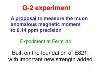
g-2
g-2. and the future of physics Student: A.C. Berceanu Supervisors: Olaf Scholten Gerco Onderwater. Theory. What does g mean?. gyromagnetic ratio =. positron charge.

g-2
E N D
Presentation Transcript
g-2 and the future of physics Student: A.C. Berceanu Supervisors: Olaf Scholten Gerco Onderwater
What does g mean? • gyromagnetic ratio = positron charge intrinsic spin angular momentum spin magnetic dipole moment mass of particle
g=2? hmm.. • Schrödinger equation postulates g=2 for pointlike leptons • Dirac equation (relativistic) actually produces the g=2 value for isolated charged, spin ½ particles (particles that just interact with an external field) • QED considers radiative corrections (a charged particle also has its own field), resulting in g values slightly larger than 2
Why is g important? • neutron: neutral! => expected g value =0 • experiment: g(neutron) = 3.82608546 • this resulted in the quark model of internal structure (total charge = 0 but contains charged sub-particles) • if CPT invariance holds then • g for the electron is known to a precision of 4ppb • CPT invariance has been tested to 10-12! • determining (fine structure constant) • testing QED • in case of the muon - constraining the SM and beyond SM physics
Anomaly • we define the anomalous magnetic moment:
Theory of leptonic g-2 Radiative corrections: muon: 99.993% electroweak contribution hadronic contribution vacuum polarization lbl scattering one loop two loops higher order vacuum polarization
The electron and its brothers muon lifetime: 2.20*10-6 s tauon lifetime: 2.96*10-13 s
Why do we like the muon? • because it’s heavy! • increased sensitivity to higher mass scale radiative corections of about 40.000! • at 0.5ppm the muon anomaly is sensitive to >100GeV scale physics
Why don’t we like the tauon that much? • after all, it’s even heavier! • the strong and weak interaction correction would be enhanced by a 1.2*107 factor • well.. yes, but its lifetime is also 10-7 times shorter compared to the muon • that makes measuring its anomalous magnetic moment almost impossible (at least for now)
What do we want to know? what needs to be calculated is the strength of a charged particle’s interaction with a magnetic field the g factor sets the strength of an electron’s interaction with a magnetic field the problem is: given a particle of know mass, charge and momentum interacting with a known magnetic field, how much will the particle’s path be deflected when it passes through the field? classical electrodynamics considers lines of magnetic flux that induce a curvature in the particle’s trajectory QED – different approach: local scattering events that can be understood in terms of Feynman diagrams
The first step.. time Feynman diagrams – purely symbolic representations of all the ways that a particular event can happen – they do NOT represent particle trajectories! space internal lines in the diagrams represent particles that cannot be observed – virtual particles; only external lines (which enter and leave the diagram) are real particles a virtual particle does not carry the same mass as its real counterpart – actually, it can have any mass whatsoever!
Feynman diagrams • external lines describe the physical process • internal lines describe the mechanism involved • first you draw all the diagrams with appropriate external lines (and different number of internal loops), then you evaluate each contribution (using conservation of energy and momentum at each vertex) and add it all up! • well, but the number of diagrams is infinite! • fortunately, each vertex introduces a factor of α, so the more loops it has the less it will contribute to the sum total
QED contribution 72 diagrams 891 diagrams 1 diagram 12,672 diagrams! 7 diagrams fine structure constant QED loops involve only virtual photons and leptons
It’s just perturbation theory! • the reason we can write this QED series expansion in the powers of the coupling constant, , is because is so small • unfortunately, as we will see in the next presentations, we cannot do that for the case of QCD, where the coupling constant is of the order of 1, so the hadronic contributions are much harder to evaluate (much harder to calculate anything with a non-perturbative theory)
The 7 two-loop diagrams vacuum polarization
Vacuum polarization • the true vacuum contains short-lived virtual particle-antiparticle pairs which are created and then annihilate each other • some of them turn out to be charged (i.e. electron – positron pairs) • such charged particles act as an electric dipole • in the presence of an electric field (eg the EM field around an electron), these particle-antiparticle pairs reposition themselves, partially counteracting the field (like a dielectric screening effect) • the field would therefore be weaker than expected when the vacuum would be completely empty
Hadronic vacuum polarization • since the particles interact strongly, the internal composition of the loop is very difficult to analyze • however, by applying dispersion theory, one can “cut in half”, giving a diagram which describes the production of real (non-virtual) hadrons • so it is possible to relate the total cross-section for hadronic production in e+e- scattering to the effect on the anomaly real hadrons
Light by light scattering • photon-photon interactions • it also occurs mediated by virtual hadrons in “hadronic light by light scattering” • this is the most difficult contribution to evaluate theoretically (one cannot apply experimental data and dispersion theory)
Most accurate QED test • in the case of the electron (for which QED corrections represent by far the main contribution) we can determine indirectly by comparing the a value with experiment • the current experimental precision in ae is 1.2ppb! • we can also determine directly (experimentally) i.e. from the quantum Hall effect • comparing the two, QED has been tested to 10-12 precision!
Cyclotron motion charged lepton with velocity moving perpendicular to uniform magnetic field
Spin precession • in the laboratory frame, the spin motion will be a uniform precession of at the spin precession frequency: precession frequency for lepton in unaccelerated motion Thomas precession due to acceleration caused by magnetic field
Putting it all together • the relative precession of with respect to will occur at a frequency: • completely independent of velocity! • one can measure g-2 directly (and gain 3 decimal places of precision for free, because g-2 is about 1/1000 of g)!
g-2 experiments • the highest experimental precision was achieved by measuring the electron g factor • this involves a single electron (or positron) moving in a trap region of high (5T) magnetic field at 4K temperature • although the classical motion of the electrons can be described as a combination of frequencies, like the muons, there are “slight” differences in the two experiments:
g-2 experiments (II) • instead of one electron we have millions of muons which contribute • the electrons have evergies in the region of 1 meV, while the muons are highly relativistic (3.1 GeV) • the electrons are trapped on cyclotron orbits of around 10-6m whereas the muons follow orbits of 7m!
Some numbers • the muons will have p=3.094 GeV/c, and this will result in a relativistic dilation of their lifetime (in the laboratory frame), from 2.2µs to 64µs • on average, they will perform 432 revolutions around the ring in one lifetime • 14.7 g-2 periods in one lifetime
The time spectrum of electrons • muon decay is a three-body decay, so they will produce a continuum of electrons from the end-point energy (3.1GeV) down • since the high energy electrons are correlated with the muon spin, if one counts hight energy electrons as a function of time one gets an exponential from muon decay modulated by the g-2 precession
The time spectrum of electrons (II) by fitting this spectrum (and making the appropriate corrections) one can get the value of , and therefore the value of the anomaly can be calculated
From an ideal g-2 experiment to a real one • the uncertainty in , where t = storage time, therefore: • requirement 1: the particle must be trapped for a long time vacuum homogenous magnetic field • requirement 2: need to measure with great precision the average magnetic field (B) “felt” by the particles (also, they must all feel the same field)
From an ideal g-2 experiment to a real one (II) • requirement 3: for maximum accuracy, the magnetic field value should be as high as possible without jeopardizing good field uniformity • the beam will have some angular divergence, so it will contain particles whose component of the velocity along the magnetic field lines is not 0! • requirement 4: focusing electric field (quadruplore field) to provide vertical focusing of the muon beam • this electric field doesn’t affect the measurement because of the “magic”
Magic gamma • with the addition of the focusing electric field, the precession frequencies become:
Conclusions • g-2 experiments on electrons represent the most stringent test of QED • g-2 of the muon is also sensitive to outside-QED (and perhaps even outside SM contributions) • muon g-2 constrained the SM for many years • an enormous amount of theoretical work continues worldwide to improve the knowledge on hadronic contributions • you will hear more about strong interactions in the upcoming presentations
Conclusions (II) • we will soon hopefully have a single SM prediction instead of two different ones! • the experimental measurements will also be improved by a factor 2 ½ over the next few years • the current discrepancy between the BNL and SM values of g-2 may indicate new physics in loop processes, internal structure of leptons or SUSY type theories, but at the present stage it is all pure speculation
Bibliography • Advanced Series on Directions in High Energy Physics – Vol. 7, “Quantum Electrodynamics”, Editor T. Kinoshita, pag. 479-504 • “QED: The strange theory of light and matter”, Richard P. Feynman,1985 • American Scientist, Vol. 92, No. 3, May-June 2004, pag. 212-216 • Hughes, V.W., and T. Kinoshita, 1999: “Anomalous g values of the electron and muon.”, Reviews of Modern Physics 71(2):S133-S139 • Muon g-2 Collaboration (G.W. Bennet et al.). Preprint. “Measurement of the negative muon anomalous magnetic moment to 0.7 ppm.” http://arxiv.org/abs/hep-ex/0401008 • Muon g-2 Collaboration (G.W. Bennet et al.) “Measurement of the positive muon anomalous magnetic moment to 0.7 ppm.” Phys. Rev. Lett. 89, 101804 (2002) • Nyffeler, Andreas. Preprint. “Theoretical status of the muon g-2.” http://arxiv.org/abs/hep-ph/0305135 • R.M. Carey et al. "An improved Muon (g-2) Experiment at J-PARC“, J-PARC Letter of Intent L17 (2003) • Arthur Rich, John C. Wesley, “The Current Status of the Lepton g Factors”, Reviews of Modern Physics, Volume 44, Number 2 • Andrzej Czarnecki, “Anomalous magnetic moments of free and bound leptons”, QED 2005, Les Houches, June 2005