V22 Modelling Dynamic Cellular Processes
V22 Modelling Dynamic Cellular Processes. Mathematical description of signalling pathways helps answering questions like: (1) How do the magnitudes of signal output and signal duration depend on the kinetic properties of pathway components?

V22 Modelling Dynamic Cellular Processes
E N D
Presentation Transcript
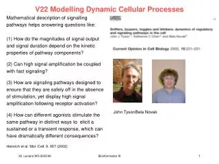
V22 Modelling Dynamic Cellular Processes Mathematical description of signalling pathways helps answering questions like: (1) How do the magnitudes of signal output and signal duration depend on the kinetic properties of pathway components? (2) Can high signal amplification be coupled with fast signaling? (3) How are signaling pathways designed to ensure that they are safely off in the absence of stimulation, yet display high signal amplification following receptor activation? (4) How can different agonists stimulate the same pathway in distinct ways to elicit a sustained or a transient response, which can have dramatically different consequences? Heinrich et al. Mol. Cell. 9, 957 (2002) John Tyson Bela Novak Bioinformatics III
The Cyclin – E2F cell cycle control system as Kohn, Molec. Biol. Cell 1999 10:2703-34 Bioinformatics III
Biocarta pathways http://cgap.nci.nih.gov/Pathways/BioCarta/h_mapkPathway Bioinformatics III
Ras signaling pathway http://cgap.nci.nih.gov/Pathways/BioCarta/h_mapkPathway Bioinformatics III
Biocarta pathways Incredible amount of information about signalling pathways! Constantly updated. How can we digest this? Need computational models! Bioinformatics III
Protein synthesis and degradation: linear response S = signal strength (e.g. concentration of mRNA) R = response magnitude (e.g. concentration of protein) A steady-state solution of a differential equation, dR/dt = f(R) is a constant Rss that satisfies the algebraic equation f(Rss) = 0. In this case Tyson et al., Curr.Pin.Cell.Biol. 15, 221 (2003) Bioinformatics III
Protein synthesis and degradation Wiring diagram rate curve signal-response curve Steady-state response R as a function of signal strength S. Solid curve: rate of removal of the response component R. Dashed lines: rates of production of R for various values of signal strength. Filled circles: steady-state solutions where rate of production and rate of removal are identical. Parameters: k0 = 0.01 k1 = 1 k2 = 5 Tyson et al., Curr.Pin.Cell.Biol. 15, 221 (2003) Bioinformatics III
phosphorylation/dephosphorylation: hyperbolic response RP: phosphorylated form of the response element RP= [RP] Pi: inorganic phosphate RT = R + RP total concentration of R Parameters: k1 = k2 = 1 RT = 1 A steady-state solution: Tyson et al., Curr.Pin.Cell.Biol. 15, 221 (2003) Bioinformatics III
phosphorylation/dephosphorylation: sigmoidal response Modification of (b) where the phosphorylation and dephosphorylation are governed by Michaelis-Menten kinetics: steady-state solution of RP The biophysically acceptable solutions must be in the range 0 < RP < RT: with the „Goldbeter-Koshland“ function G: Tyson et al., Curr.Pin.Cell.Biol. 15, 221 (2003) Bioinformatics III
phosphorylation/dephosphorylation: sigmoidal response This mechanism creates a switch-like signal-response curve which is called zero-order ultrasensitivity. (a), (b), and (c) give „graded“ and reversible behavior of R and S. „graded“: R increases continuously with S reversible: if S is change from Sinitial to Sfinal , the response at Sfinal is the same whether the signal is being increased (Sinitial < Sfinal) or decreased (Sinitial > Sfinal). Element behaves like a buzzer: to activate the response, one must push hard enough on the button. Parameters: k1 = k2 = 1 RT = 1 Km1 = Km2 = 0.05 Tyson et al., Curr.Pin.Cell.Biol. 15, 221 (2003) Bioinformatics III
perfect adaptation: sniffer Here, the simple linear response element is supplemented with a second signaling pathway through species X. The response mechanism exhibits perfect adaptation to the signal: although the signaling pathway exhibits a transient response to changes in signal strength, its steady-state response Rssis independent of S. Such behavior is typical of chemotactic systems, which respond to an abrupt change in attractants or repellents, but then adapt to a constant level of the signal. Our own sense of smell operates this way we call this element „sniffer“. Tyson et al., Curr.Pin.Cell.Biol. 15, 221 (2003) Bioinformatics III
Parameters: k1 = k2 = 2 k3 = k4 = 1 perfect adaptation Right panel: transient response (R, black) as a function of stepwise increases in signal strength S (red) with concomitant changes in the indirect signaling pathway X (green). The signal influences the response via two parallel pathways that push the response in opposite directions. This is an example of feed-forward control. Alternatively, some component of a response pathway may feed back on the signal (positive, negative, or mixed). Tyson et al., Curr.Opin.Cell.Biol. 15, 221 (2003) Bioinformatics III
Positive feedback: Mutual activation E: a protein involved with R EP: phosphorylated form of E Here, R activates E by phosphorylation, and EP enhances the synthesis of R. Tyson et al., Curr.Opin.Cell.Biol. 15, 221 (2003) Bioinformatics III
mutual activation: one-way switch As S increases, the response is low until S exceeds a critical value Scrit at which point the response increases abruptly to a high value. Then, if S decreases, the response stays high. between 0 and Scrit, the control system is „bistable“ – it has two stable steady-state response values (on the upper and lower branches, the solid lines) separated by an unstable steady state (on the intermediate branch, the dashed line). This is called a one-parameter bifurcation. Tyson et al., Curr.Opin.Cell.Biol. 15, 221 (2003) Bioinformatics III
mutual inhibition Here, R inhibits E, and E promotes the degradation of R. Tyson et al., Curr.Opin.Cell.Biol. 15, 221 (2003) Bioinformatics III
mutual inhibition: toggle switch This bifurcation is called toggle switch („Kippschalter“): if S is decreased enough, the switch will go back to the off-state. For intermediate stimulus strengh (Scrit1 < S < Scrit2), the response of the system can be either small or large, depending on how S was changed. This is often called „hysteresis“. Examples: lac operon in bacteria, activation of M-phase promoting factor in frog egg extracts, and the autocatalytic conversion of normal prion protein to its pathogenic form. Tyson et al., Curr.Opin.Cell.Biol. 15, 221 (2003) Bioinformatics III
Negative feedback: homeostasis In negative feedback, the response counteracts the effect of the stimulus. Here, the response element R inhibits the enzyme E catalyzing its synthesis. Therefore, the rate of production of R is a sigmoidal decreasing function of R. Negative feedback in a two-component system X R | X can also exhibit damped oscillations to a stable steady state but not sustained oscillations. Tyson et al., Curr.Opin.Cell.Biol. 15, 221 (2003) Bioinformatics III
Negative feedback: oscillatory response Sustained oscillations require at least 3 components: X Y R |X Left: example for a negative-feedback control loop. There are two ways to close the negative feedback loop: (1) RP inhibits the synthesis of X (2) RP activates the degradation of X. Tyson et al., Curr.Opin.Cell.Biol. 15, 221 (2003) Bioinformatics III
Negative feedback: oscillatory response Feedback loop leads to oscillations of X (black), YP (red), and RP (blue). Within the range Scrit1 < S < Scrit2, the steady-state response RP,ss is unstable. Within this range, RP(t) oscillates between RPmin and RPmax. Again, Scrit1 and Scrit2 are bifurcation points. The oscillations arise by a generic mechanism called „Hopf bifurcation“. Negative feedback has ben proposed as a basis for oscillations in protein synthesis, MPF activity, MAPK signaling pathways, and circadian rhythms. Tyson et al., Curr.Pin.Cell.Biol. 15, 221 (2003) Bioinformatics III
Positive and negative feedback: Activator-inhibitor oscillations R is created in an autocatalytic process, and then promotes the production of an inhibitor X, which speeds up R removal. The classic example of such a system is cyclic AMP production in the slime mold. External cAMP binds to a surface receptor, which stimulates adenylate cyclase to produce and excrete more cAMP. At the same time, cAMP-binding pushes the receptor into an inactive form. After cAMP falls off, the inactive form slowly recovers its ability to bind cAMP and stimulate adenylate cyclase again. Tyson et al., Curr.Pin.Cell.Biol. 15, 221 (2003) Bioinformatics III
Substrate-depletion oscillations X is converted into R in an autocatalytic process. Suppose at first, X is abundant and R is scarce. As R builds up, the production of R accelerates until there is an explosive conversion of the entire pool of X into R. Then, the autocatalytic reaction shuts off for lack of substrate, X. R is degraded, and X must build up again. This is the mechanism of MPF oscillations in frog egg extract. Tyson et al., Curr.Pin.Cell.Biol. 15, 221 (2003) Bioinformatics III
Complex networks All the signal-response elements just described, buzzers, sniffers, toggles and blinkers, usually appear as components of more complex networks. Example: wiring diagram for the Cdk network regulating DNA synthesis and mitosis. The network involving proteins that regulate the activity of Cdk1-cyclin B heterodimers consists of 3 modules that oversee the - G1/S - G2/M, and - M/G1 transitions of the cell cycle. Tyson et al., Curr.Pin.Cell.Biol. 15, 221 (2003) Bioinformatics III
Cell cycle control system Tyson et al., Curr.Pin.Cell.Biol. 15, 221 (2003) Bioinformatics III
Cell cycle control system The G1/S module is a toggle switch, based on mutual inhibition between Cdk1-cyclin B and CKI, a stoichiometric cyclin-dependent kinase inhibitor. Tyson et al., Curr.Pin.Cell.Biol. 15, 221 (2003) Bioinformatics III
Cell cycle control system The G2/M module is a second toggle switch, based on mutual activation between Cdk1-cyclinB and Cdc25 (a phosphotase that activates the dimer) and mutual inhibition between Cdk1-cyclin B and Wee1 (a kinase that inactivates the dimer). Tyson et al., Curr.Pin.Cell.Biol. 15, 221 (2003) Bioinformatics III
Cell cycle control system The M/G1 module is an oscillator, based on a negative-feedback loop: Cdk1-cyclin B activates the anaphase-promoting complex (APC), which activates Cdc20, which degrades cyclin B. The „signal“ that drives cell proliferation is cell growth: a newborn cell cannot leave G1 and enter the DNA synthesis/division process (S/G2/M) until it grows to a critical size. Tyson et al., Curr.Pin.Cell.Biol. 15, 221 (2003) Bioinformatics III
Cell cycle control system The signal-response curve is a plot of steady-state activity of Cdk1-cyclin B as a function of cell size. Progress through the cell cycle is viewed as a sequence of bifurcations. A very small newborn cell is attracted to the stable G1 steady state. As it grows, it eventually passes the saddle-point bifurcation SN3 where the G1 steady state disappears. The cell makes an irreversible transition into S/G2 until it grows so large that the S/G2 steady state disappears, giving way to an infite period oscillation (SN/IP). Cyclin-B-dependent kinase activity soars, driving the cell into mitosis, and then plummets, as cyclin B is degraded by APC–Cdc20. The drop in Cdk1–cyclin B activity is the signal for the cell to divide, causing cell size to be halved from 1.46 to 0.73, and the control system is returned to its starting point, in the domain of attraction of the G1 steady state. Tyson et al., Curr.Pin.Cell.Biol. 15, 221 (2003) Bioinformatics III