Download
1 / 82
970 likes | 1.74k Vues
Signals & systems Ch.3 Fourier Transform of Signals and LTI System. Signals and systems in the Frequency domain. Fourier transform. Time [sec]. Frequency [sec -1 , Hz]. 3.1 Introduction. Orthogonal vector => orthonomal vector What is meaning of magnitude of H?.

E N D
Signals & systemsCh.3 Fourier Transform of Signals and LTI System
Signals and systems in the Frequency domain Fourier transform Time [sec] Frequency [sec-1, Hz] KyungHee University
3.1 Introduction • Orthogonal vector => orthonomal vector • What is meaning of magnitude of H? Any vector in the 2- dimensional space can be represented by weighted sum of 2 orthonomal vectors Fourier Transform(FT) Inverse FT KyungHee University
3.1 Introduction cont’ • CDMA? Orthogonal? Any vector in the 4- dimensional space can be represented by weighted sum of 4 orthonomal vectors Orthonormal function? KyungHee University
3.1 Introduction cont’ • Fourier Series (FS) i) If ii) If Any periodic function(signal) with period T can be represented by weighted sum of orthonormal functions. What is meaning of magnitude of Fk? Think about equalizer in audio system. KyungHee University
3.2 Complex Sinusoids and Frequency Response of LTI Systems cf) impulse response How about for complex z? (3.1) How about for complex s? (3.3) Magnitude to kill or not? Phase delay KyungHee University
3.3 Fourier Representations for Four Classes of signals • 3.3.1 Periodic Signals: Fourier Series Representations “Any periodic function can be represented by weighted sum of basic periodic function.” Fourier said (periodic) - (discrete) (discrete) - (periodic) DTFS (3.4) CTFS (3.5) Periodic? yes! With the period of N KyungHee University
3.3 Fourier Representations for Four Classes of signals cont’ • 3.3.2 Non-periodic Signals: Fourier-Transform Representations (aperiodic) - (continuous) (continuous) - (aperiodic) Inverse continuous time Fourier Transform (CTFT) (aperiodic) - (continuous) (discrete) - (periodic) Inverse discrete time Fourier Transform (DTFT) KyungHee University
3.4 Discrete-Time Periodic Signals: The Discrete-Time Fourier Series (periodic) - (discrete) (discrete) - (periodic) Inverse DFT (3.10) DFT Example 3.2 Determining DTFS Coefficients Figure 3.5 Time-domain signal for Example 3.2. Find the frequency-domain representation of the signal depicted in Fig. 3.5 KyungHee University
3.4 Discrete-Time Periodic Signals: The Discrete-Time Fourier Series cont’ Just inner product to orthonormal vectors in the 5 dimensional space!! KyungHee University
3.4 Discrete-Time Periodic Signals: The Discrete-Time Fourier Series cont’ DC!! Figure 3.6 Magnitude and phase of the DTFS coefficients for the signal in Fig. 3.5. Recall “weighted sum of orthonormal vectors in the 5 dimensional space” KyungHee University
3.4 Discrete-Time Periodic Signals: The Discrete-Time Fourier Series cont’ Example 3.3 Computation of DTFS Coefficients by Inspection orthnormal Determine the DTFS coefficients of , using the method of inspection. Figure 3.8 Magnitude and phase of DTFS coefficients for Example 3.3. KyungHee University
3.4 Discrete-Time Periodic Signals: The Discrete-Time Fourier Series cont’ Example 3.4 DTFS Representation of an Impulse Train Find the DTFS Coefficients of the N-periodic impulse train Figure 3.9 A discrete-time impulse train with period N. How about in other period? Draw X[k] in the k-axis. (impulse train) - (impulse train) KyungHee University
3.4 Discrete-Time Periodic Signals: The Discrete-Time Fourier Series cont’ Example 3.5 The Inverse DTFS of periodic X[k] Use Eq. (3.10) to determine the time-domain signal x[n] from the DTFS coefficients depicted in Fig. 3.10 Figure 3.10 Magnitude and phase of DTFS coefficients for Example 3.5. KyungHee University
3.4 Discrete-Time Periodic Signals: The Discrete-Time Fourier Series cont’ Example 3.6 DTFS Representation of a Square Wave Find the DTFS coefficients for the N-periodic square wave Figure 3.11 Square wave for Example 3.6. (3.15) 등비수열의 합 DC=mean=평균 KyungHee University
3.4 Discrete-Time Periodic Signals: The Discrete-Time Fourier Series cont’ DC, also Then for all k. M=0 (impulse train) 2M+1 = N? (square) -(sinc) KyungHee University
3.4 Discrete-Time Periodic Signals: The Discrete-Time Fourier Series cont’ Example 3.7 Building a Square Wave form DTFS Coefficients symmetric Evaluate one period of the Jth term in Eq. (3.18) and the 2J+1 term approximation for J=1, 3, 5, 23, and 25. (3.18) KyungHee University
3.4 Discrete-Time Periodic Signals: The Discrete-Time Fourier Series cont’ Example 3.8 Numerical Analysis of the ECG Evaluate the DTFS representations of the two electrocardiogram (ECG) waveforms depicted in Figs. 3.15(a) and (b). • Normal heartbeat. • Ventricular tachycardia. • Magnitude spectrum for the normal heartbeat. • Magnitude spectrum for ventricular tachycardia. Figure 3.15 Electrocardiograms for two different heartbeats and the first 60 coefficients of their magnitude spectra. KyungHee University
3.5 Continuous-Time Periodic Signals: The Fourier Series Any periodic function can be represented by weighted sum of basic periodic functions. (periodic) (discrete) (continuous) (aperiodic) Inverse FT where (3.19) Recall “orthonormal”!! FT (3.20) KyungHee University
3.5 Continuous-Time Periodic Signals: The Fourier Series cont’ Example 3.9 Direct Calculation of FS Coefficients Determine the FS coefficients for the signal depicted in Fig. 3. 16. Solution : X[0]=? FT Figure 3.16 Time-domain signal for Example 3.9. Figure 3.17 Magnitude and phase for Ex. 3.9. KyungHee University
3.5 Continuous-Time Periodic Signals: The Fourier Series cont’ Example 3.10 FS Coefficients for an Impulse Train. Determine the FS coefficients for the signal defined by Solution : (impulse train) (impulse train) Example 3.11 Calculation of FS Coefficients by Inspection Determine the FS representation of the signal using the method of inspection. Solution : (3.21) (3.22) Figure 3.18 Magnitude and phase for Ex. 3.11. KyungHee University
3.5 Continuous-Time Periodic Signals: The Fourier Series cont’ Example 3.12 Inverse FS : Find the time-domain signal x(t) corresponding to the FS coefficients . Assume that the fundamental period is Solution : 등비수열의 합 Figure 3.20 FS coefficients for Problem 3.9. Figure 3.21 Square wave for Example 3.13. KyungHee University
3.5 Continuous-Time Periodic Signals: The Fourier Series cont’ Example 3.13 FS for a Square Wave Determine the FS representation of the square wave depicted in Fig. 3.21. For k=0, where Figure 3.22 The FS coefficients, X[k], –50 k 50, for three square waves. In Fig. 3.21 Ts/T = (a) 1/4 . (b) 1/16. (c) 1/64. KyungHee University
3.5 Continuous-Time Periodic Signals: The Fourier Series cont’ To/T=1/2? (DC) (impulse) To 0? (impulse train) (impulse train) T ? (aperiodic) (continuous) (square) (sinc) (sinc) (square) Figure 3.23 Sinc function sinc(u) = sin(u)/(u) KyungHee University
3.5 Continuous-Time Periodic Signals: The Fourier Series cont’ Example 3.14 Square-Wave Partial-Sum Approximation Let the partial-sum approximation to the FS in Eq.(3.29), be given by This approximation involves the exponential FS Coefficients with indices . Consider a square wave and . Depict one period of the th term in this sum, and find for and 99. Solution : KyungHee University
3.6 Discrete-Time Non-periodic Signals : The Discrete-Time Fourier Transform (discrete) (periodic) (3.31) (3.32) KyungHee University
3.6 Discrete-Time Non-periodic Signals : The Discrete-Time Fourier Transform cont’ Example 3.17 DTFT of an Exponential Sequence Find the DTFT of the sequence Solution : = 0.5 = 0.9 x[n] = nu[n]. magnitude = 0.5 = 0.9 phase KyungHee University
3.6 Discrete-Time Non-periodic Signals : The Discrete-Time Fourier Transform cont’ Example 3.18 DTFT of a Rectangular Pulse Let Find the DTFT of Solution : (square) (sinc) Figure 3.30 Example 3.18. (a) Rectangular pulse in the time domain. (b) DTFT in the frequency domain. KyungHee University
3.6 Discrete-Time Non-periodic Signals : The Discrete-Time Fourier Transform cont’ KyungHee University
3.6 Discrete-Time Non-periodic Signals : The Discrete-Time Fourier Transform cont’ Example 3.19 Inverse DTFT of a Rectangular Spectrum Find the inverse DTFT of Solution : (sinc) (square) Figure 3.31 (a) Rectangular pulse in the frequency domain. (b) Inverse DTFT in the time domain. KyungHee University
3.6 Discrete-Time Non-periodic Signals : The Discrete-Time Fourier Transform cont’ Example 3.20 DTFT of the Unit Impulse Find the DTFT of Solution : (impulse) - (DC) Example 3.21 Find the inverse DTFT of a Unit Impulse Spectrum. Solution : (impulse train) (impulse train) KyungHee University
3.6 Discrete-Time Non-periodic Signals : The Discrete-Time Fourier Transform cont’ Example 3.22 Two different moving-average systems solution : Figure 3.36 KyungHee University
3.6 Discrete-Time Non-periodic Signals : The Discrete-Time Fourier Transform cont’ Example 3.23 Multipath Channel : Frequency Response Solution : (a) a = 0.5ej2/3. (b) a = 0.9ej2/3. (a) a = 0.5ej2/3. (b) a = 0.9ej2/3. KyungHee University
3.7 Continuous-Time Non-periodic Signals : The Fourier Transform (continuous aperiodic) (continuous aperiodic) Inverse CTFT (3.35) CTFT (3.26) Condition for existence of Fourier transform: KyungHee University
3.7 Continuous-Time Non-periodic Signals : The Fourier Transform cont’ Example 3.24 FT of a Real Decaying Exponential Find the FT of Solution : Therefore, FT not exists. LPF or HPF? Cut-off from 3dB point? KyungHee University
3.7 Continuous-Time Non-periodic Signals : The Fourier Transform cont’ Example 3.25 FT of a Rectangular Pulse Find the FT of x(t). Solution : (square) (sinc) Example 3.25. (a) Rectangular pulse. (b) FT. KyungHee University
3.7 Continuous-Time Non-periodic Signals : The Fourier Transform cont’ Example 3.26 Inverse FT of an Ideal Low Pass Filter!! Fine the inverse FT of the rectangular spectrum depicted in Fig.3.42(a) and given by Solution : (sinc) -- (square) KyungHee University
3.7 Continuous-Time Non-periodic Signals : The Fourier Transform cont’ Example 3.27 FT of the Unit Impulse Solution : (impulse) - (DC) Example 3.28 Inverse FT of an Impulse Spectrum Find the inverse FT of Solution : (DC) (impulse) KyungHee University
3.7 Continuous-Time Non-periodic Signals : The Fourier Transform cont’ Example 3.29 Digital Communication Signals Rectangular (wideband) Separation between KBS and SBS. Narrow band Figure 3.44 Pulse shapes used in BPSK communications. (a) Rectangular pulse. (b) Raised cosine pulse. KyungHee University
3.7 Continuous-Time Non-periodic Signals : The Fourier Transform cont’ Solution : Figure 3.45 BPSK (a) rectangular pulse shapes (b) raised-cosine pulse shapes. the same power constraints KyungHee University
3.7 Continuous-Time Non-periodic Signals : The Fourier Transform cont’ rectangular pulse. One sinc Raised cosine pulse 3 sinc’s The narrower main lobe, the narrower bandwidth. But, the more error rate as shown in the time domain Figure 3.47 sum of three frequency-shifted sinc functions. KyungHee University
9.1 Linearity and Symmetry Properties of FT KyungHee University
9.1 Linearity and Symmetry Properties of FT cont’ • 3.9.1 Symmetry Properties : Real and Imaginary Signals (3.37) (real x(t)=x*(t)) (conjugate symmetric) (3.38) KyungHee University
9.1 Linearity and Symmetry Properties of FT cont’ • 3.9.2 SYSMMEYRY PROPERTIES : EVEN/ODD SIGNALS (even) (real) (odd) (pure imaginary) For even x(t), real KyungHee University
3.10 Convolution Property • 3.10.1 CONVOLUTION OF NON-PERIODIC SIGNALS (convolution) (multiplication) But given change the order of integration KyungHee University
3.10 Convolution Property cont’ Example 3.31 Convolution problem in the frequency domain be the input to a system with impulse response Find the output Solution: KyungHee University
3.10 Convolution Property cont’ Example 3.32 Find inverse FT’S by the convolution property Use the convolution property to find , where Ex 3.32 (p. 261). (a) Rectangular z(t). (b) KyungHee University
3.10 Convolution Property cont’ • 3.10.2 FILTERING Continuous time Discrete time LPF HPF BPF Figure 3.53 (p. 263) Frequency dependent gain (power spectrum) kill or not (magnitude) KyungHee University
3.10 Convolution Property cont’ Example 3.34 Identifying h(t) from x(t) and y(t) The output of an LTI system in response to an input is . Find frequency response and the impulse response of this system. Solution: But KyungHee University
3.10 Convolution Property cont’ EXAMPLE 3.35 Equalization of multipath channel or Consider again the problem addressed in Example 2.13. In this problem, a distorted received signal y[n] is expressed in terms of a transmitted signal x[n] as Then KyungHee University