Maximizing Bandwidth Utilization in Data Communications
Explore the efficient utilization of limited bandwidth in electronic communications through multiplexing techniques like Frequency-Division Multiplexing. Learn how to share bandwidth among devices and maximize resource usage.

Maximizing Bandwidth Utilization in Data Communications
E N D
Presentation Transcript
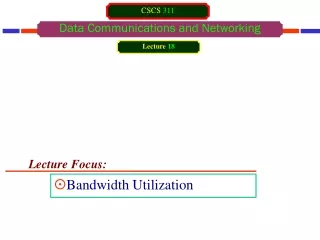
Lecture Focus: Bandwidth Utilization CSCS 311 Data Communications and Networking Lecture 18
Bandwidth Utilization • In real life, we have links with limited bandwidths. • The wise use of these bandwidths has been, and will be, one of the main challenges of electronic communications. • Sometimes we need to combine several low-bandwidth channels to make use of one channel with a larger bandwidth. • Sometimes we need to expand the bandwidth of a channel to achieve goals such as privacy and anti-jamming. • There are two broad categories of bandwidth utilization: • Multiplexing • In multiplexing, our goal is efficiency; • We combine several channels into one. • Spreading • In spreading, our goals are privacy and anti-jamming; • We expand the bandwidth of a channel • Efficiency can be achieved by multiplexing; • Privacy and anti-jamming can be achieved by spreading.
Bandwidth Utilization MULTIPLEXING • Whenever the bandwidth of a medium linking two devices is greater than the bandwidth needs of the devices, the link can be shared. • Multiplexing is the set of techniques that allows the simultaneous transmission of multiple signals across a single data link. • As data and telecommunications use increases, so does traffic. • We can accommodate this increase by continuing to add individual links each time a new channel is needed; or • We can install higher-bandwidth links and use each to carry multiple signals. • Today's technology includes high-bandwidth media such as optical fiber and terrestrial and satellite microwaves. • Each has a bandwidth far in excess of that needed for the average transmission signal. • If the bandwidth of a link is greater than the bandwidth needs of the devices connected to it, the bandwidth is wasted. • An efficient system maximizes the utilization of all resources; bandwidth is one of the most precious resources we have in data communications.
Bandwidth Utilization MULTIPLEXING • In a multiplexed system, n lines share the bandwidth of one link. • Figure below shows the basic format of a multiplexed system. • The lines on the left direct their transmission streams to a multiplexer (MUX), which combines them into a single stream (many-to-one). • At the receiving end, that stream is fed into a demultiplexer (DEMUX), which separates the stream back into its component transmissions (one-to-many) and directs them to their corresponding lines. • In the figure, the word link refers to the physical path. The word channel refers to the portion of a link that carries a transmission between a given pair of lines. • One link can have many (n) channels.
Bandwidth Utilization MULTIPLEXING Dividing a link into n channels
Bandwidth Utilization MULTIPLEXING Dividing a link into 4 channels
Bandwidth Utilization MULTIPLEXING Categories of multiplexing • There are three basic multiplexing techniques: • Frequency-division multiplexing • Wavelength-division multiplexing • Time-division multiplexing • The first two are techniques designed for analog signals, the third, for digital signals.
MULTIPLEXING Categories of multiplexing Frequency-Division Multiplexing (FDM) • Frequency-division multiplexing (FDM) is an analog technique that can be applied when the bandwidth of a link (in hertz) is greater than the combined bandwidths of the signals to be transmitted. • In FDM, signals generated by each sending device modulate different carrier frequencies. • These modulated signals are then combined into a single composite signal that can be transported by the link. • Carrier frequencies are separated by sufficient bandwidth to accommodate the modulated signal. • These bandwidth ranges are the channels through which the various signals travel.
MULTIPLEXING Categories of multiplexing Frequency-Division Multiplexing (FDM) • Channels can be separated by strips of unused bandwidth to prevent signals from overlapping. • These strips of unused bandwidth are called guard bands. • In addition, carrier frequencies must not interfere with the original data frequencies. • Figure below gives a conceptual view of FDM. • In this illustration, the transmission path is divided into three parts, each representing a channel that carries one transmission.
MULTIPLEXING Categories of multiplexing Frequency-Division Multiplexing (FDM) • FDM is considered to be an analog multiplexing technique; however, this does not mean that FDM cannot be used to combine sources sending digital signals. • A digital signal can be converted to an analog signal before FDM is used to multiplex them. FDM is an analog multiplexing technique that combines analog signals.
MULTIPLEXING Categories of multiplexing Frequency-Division Multiplexing (FDM) Multiplexing Process • Figure below is a conceptual illustration of the multiplexing process. • Each source generates a signal of a similar frequency range. • Inside the multiplexer, these similar signals modulates different carrier frequencies (f1,f2, and f3). • The resulting modulated signals are then combined into a single composite signal that is sent out over a media link that has enough bandwidth to accommodate it.
MULTIPLEXING Categories of multiplexing Frequency-Division Multiplexing (FDM) De-Multiplexing Process • The demultiplexer uses a series of filters to decompose the multiplexed signal into its constituent component signals. • The individual signals are then passed to a demodulator that separates them from their carriers and passes them to the output lines. • Figure below is a conceptual illustration of de-multiplexing process.
MULTIPLEXING Categories of multiplexing Frequency-Division Multiplexing (FDM) De-Multiplexing Process Assume that a voice channel occupies a bandwidth of 4 KHz. We need to combine three voice channels into a link with a bandwidth of 12 KHz, from 20 to 32 KHz. Show the configuration using the frequency domain without the use of guard bands. Example Solution Shift (modulate) each of the three voice channels to a different bandwidth. We shift (modulate) each of the three voice channels to a different bandwidth. We use the 20- to 24-kHz bandwidth for the first channel, the 24- to 28-kHz bandwidth for the second channel, and the 28- to 32-kHz bandwidth for the third one. Then we combine them. At the receiver, each channel receives the entire signal, using a filter to separate out its own signal. The first channel uses a filter that passes frequencies between 20 and 24 kHz and filters out (discards) any other frequencies. The second channel uses a filter that passes frequencies between 24 and 28 kHz, and the third channel uses a filter that passes frequencies between 28 and 32 kHz. Each channel then shifts the frequency to start from zero.
MULTIPLEXING Categories of multiplexing Frequency-Division Multiplexing (FDM) Multiplexing and De-Multiplexing Process
MULTIPLEXING Categories of multiplexing Frequency-Division Multiplexing (FDM) De-Multiplexing Process Example Five channels, each with a 100-KHz bandwidth, are to be multiplexed together. What is the minimum bandwidth of the link if there is a need for a guard band of 10 KHz between the channels to prevent interference? For five channels, we need at least four guard bands. This means that the required bandwidth is at least 5 x 100 + 4 x 10 = 540 KHz. Solution
MULTIPLEXING Categories of multiplexing Frequency-Division Multiplexing (FDM) The Analog Carrier System or Analog Hierarchy • To maximize the efficiency of their infrastructure, telephone companies have traditionally multiplexed signals from lower-bandwidth lines onto higher-bandwidth lines. • In this way, many switched or leased lines can be combined into fewer but bigger channels. • For analog lines, FDM is used. • One of these hierarchical systems used by AT&T is made up of groups, super-groups, master groups, and jumbo groups.
MULTIPLEXING Categories of multiplexing Frequency-Division Multiplexing (FDM) The Analog Carrier System or Analog Hierarchy • In this analog hierarchy, 12 voice channels are multiplexed onto a higher-bandwidth line to create a group. A group has 48 kHz of bandwidth and supports 12 voice channels. • At the next level, up to five groups can be multiplexed to create a composite signal called a super-group. A super-group has a bandwidth of 240 kHz and supports up to 60 voice channels. Super-groups can be made up of either five groups or 60 independent voice channels. • At the next level, 10 super-groups are multiplexed to create a master group. A master group must have 2.40 MHz of bandwidth, but the need for guard bands between the super-groups increases the necessary bandwidth to 2.52 MHz. • Master groups support up to 600 voice channels. • Finally, six master groups can be combined into a jumbo group. A jumbo group must have 15.12 MHz (6 x 2.52 MHz) but is augmented to 16.984 MHz to allow for guard bands between the master groups.
MULTIPLEXING Categories of multiplexing Frequency-Division Multiplexing (FDM) The Analog Carrier System or Analog Hierarchy
MULTIPLEXING Categories of multiplexing Frequency-Division Multiplexing (FDM) Applications of FDM: Radio Broadcasting • A very common application of FDM is AM and FM radio broadcasting. • Radio uses the air as the transmission medium. • A special band from 530 to 1700 kHz is assigned to AM radio. • All radio stations need to share this band. • Each AM station needs 10kHz of bandwidth. • Each station uses a different carrier frequency, which means it is shifting its signal and multiplexing. • The signal that goes to the air is a combination of signals. • A receiver receives all these signals, but filters (by tuning) only the one which is desired. • Without multiplexing, only one AM station could broadcast to the common link, the air. However, there is physical multiplexer or demultiplexer here. • Multiplexing is done at the data link layer. • Situation is similar in FM broadcasting. However, FM has a wider band of 88 to 108 MHz because each station needs a bandwidth of 200 kHz.
MULTIPLEXING Categories of multiplexing Frequency-Division Multiplexing (FDM) Applications of FDM: Television Broadcasting • Another common use of FDM is in television broadcasting. • Each TV channel has its own bandwidth of 6 MHz. Applications of FDM: Cellular Telephones • The first generation of cellular telephones (still in operation) also uses FDM. • Each user is assigned two 30-kHz channels, one for sending voice and the other for receiving. • The voice signal, which has a bandwidth of 3 kHz (from 300 to 3300 Hz), is modulated by using FM. • Remember that an FM signal has a bandwidth 10 times that of the modulating signal, which means each channel has 30 kHz (10 x 3) of bandwidth. • Therefore, each user is given, by the base station, a 60-kHz bandwidth in a range available at the time of the call.
MULTIPLEXING Categories of multiplexing Frequency-Division Multiplexing (FDM) Applications of FDM: Television Broadcasting Example The Advanced Mobile Phone System (AMPS) uses two bands. The first band, 824 to 849 MHz, is used for sending; and 869 to 894 MHz is used for receiving. Each user has a bandwidth of 30 KHz in each direction. The 3-KHz voice is modulated using FM, creating 30 KHz of modulated signal. How many people can use their cellular phones simultaneously? Solution Each band is 25 MHz. If we divide 25 MHz into 30 KHz, we get 833.33. In reality, the band is divided into 832 channels. Of these, 42 channels are used for control. It means only 790 channels are available for cellular phone users.
MULTIPLEXING Categories of multiplexing Frequency-Division Multiplexing (FDM) Implementation • FDM can be implemented very easily. • In many cases, such as radio and television broadcasting, there is no need for a physical multiplexer or demultiplexer. • As long as the stations agree to send their broadcasts to the air using different carrier frequencies, multiplexing is achieved. • In the cellular telephone system, a base station needs to assign a carrier frequency to the telephone user. • There is not enough bandwidth in a cell to permanently assign a bandwidth range to every telephone user. • When a user hangs up, his/her bandwidth is assigned to another caller.
MULTIPLEXING Categories of multiplexing Wavelength-Division Multiplexing (WDM) • Wavelength-division multiplexing (WDM) is designed to use the high-data-rate capability of fiber-optic cable. • The optical fiber data rate is higher than the data rate of metallic transmission cable. • Using a fiber-optic cable for one single line wastes the available bandwidth. • Multiplexing allows us to combine several lines into one. • WDM is conceptually the same as FDM, except that the multiplexing and de-multiplexing involve optical signals transmitted through fiber-optic channels. • The idea is the same: • We are combining different signals of different frequencies. • The difference is that the frequencies are very high.
MULTIPLEXING Categories of multiplexing Wavelength-Division Multiplexing (WDM) • Figure below gives a conceptual view of a WDM multiplexer and demultiplexer. • Very narrow bands of light from different sources are combined to make a wider band of light. • At the receiver, the signals are separated by the demultiplexer. WDM is an analog multiplexing technique to combine optical signals.
MULTIPLEXING Categories of multiplexing Wavelength-Division Multiplexing (WDM) • Although WDM technology is very complex, the basic idea is very simple. • We combine multiple light sources into one single light at the multiplexer and do the reverse at the demultiplexer. • The combining and splitting of light sources are easily handled by a prism. • A prism bends a beam of light based on the angle of incidence and the frequency. • Using this technique, a multiplexer can be made to combine several input beams of light, each containing a narrow band of frequencies, into one output beam of a wider band of frequencies. • A demultiplexer can also be made to reverse the process. • Figure below shows the concept.
MULTIPLEXING Categories of multiplexing Wavelength-Division Multiplexing (WDM) Prisms in wavelength-division multiplexing and de-multiplexing
MULTIPLEXING Categories of multiplexing Time-Division Multiplexing (TDM) • Time-division multiplexing (TDM) is a digital process that allows several connections to share the high bandwidth of a link. • Instead of sharing a portion of the bandwidth as in FDM, time is shared. • Each connection occupies a portion of time in the link. • Figure below gives a conceptual view of TDM. • In the figure, portions of signals 1,2,3, and 4 occupy the link sequentially.
MULTIPLEXING Categories of multiplexing Time-Division Multiplexing (TDM) • We can divide TDM into two different schemes: • Synchronous • Statistical
MULTIPLEXING Categories of multiplexing Time-Division Multiplexing (TDM) Synchronous TDM • In synchronous TDM, each input connection has an allotment in the output even if it is not sending data. Time Slots and Frames • In synchronous TDM, the data flow of each input connection is divided into units, where each input occupies one input time slot. • A unit can be 1 bit, one character, or one block of data. • Each input unit becomes one output unit and occupies one output time slot. • However, the duration of an output time slot is n times shorter than the duration of an input time slot. • If an input time slot is T sec, the output time slot is T/n sec, where n is the number of connections. • In other words, a unit in the output connection has a shorter duration; it travels faster.
MULTIPLEXING Categories of multiplexing Time-Division Multiplexing (TDM) Synchronous TDM • In synchronous TDM, a round of data units from each input connection is collected into a frame. • If we have n connections, a frame is divided into n time slots and one slot is allocated for each unit, one for each input line. • If the duration of the input unit is T, the duration of each slot is T/n and the duration of each frame is T (unless a frame carries some other information). • Time slots are grouped into frames. • A frame consists of one complete cycle of time slots, with one slot dedicated to each sending device. • In a system with n input lines, each frame has n slots, with each slot allocated to carrying data from a specific input line.
MULTIPLEXING Categories of multiplexing Time-Division Multiplexing (TDM) Synchronous TDM Time Slots and Frames • Example of synchronous TDM where n is 3. Figure : ABC
MULTIPLEXING Categories of multiplexing Time-Division Multiplexing (TDM) Synchronous TDM Interleaving • TDM can be visualized as two fast-rotating switches, one on the multiplexing side and the other on the de-multiplexing side. • The switches are synchronized and rotate at the same speed, but in opposite directions. • On the multiplexing side, as the switch opens in front of a connection, that connection has the opportunity to send a unit onto the path. This process is called interleaving.
MULTIPLEXING Categories of multiplexing Time-Division Multiplexing (TDM) Interleaving Synchronous TDM • On the de-multiplexing side, as the switch opens in front of a connection, that connection has the opportunity to receive a unit from the path. • Figure on next slide shows the interleaving process for the connection shown in Figure ABC (previously shown). • In this figure, we assume that no switching is involved and that the data from the first connection at the multiplexer site go to the first connection at the demultiplexer. Figure : ABC
MULTIPLEXING Categories of multiplexing Time-Division Multiplexing (TDM) Synchronous TDM Interleaving
MULTIPLEXING Categories of multiplexing Time-Division Multiplexing (TDM) Synchronous TDM Example Four channels are multiplexed using TDM. If each channel sends 100 bytes/s and we multiplex 1 byte per channel, show the frame traveling on the link, the size of the frame, the duration of a frame, the frame rate, and the bit rate for the link. Solution The multiplexer is shown below. Each frame carries 1 byte from each channel; the size of each frame, therefore, is 4 bytes, or 32 bits. Because each channel is sending 100 bytes/s and a frame carries 1 byte from each channel, the frame rate must be 100 frames per second. The duration of a frame is therefore 1/100 s. The link is carrying 100 frames per second, and since each frame contains 32 bits, the bit rate is 100 x 32, or 3200 bps. This is actually 4 times the bit rate of each channel, which is 100 x 8 =800 bps.
MULTIPLEXING Categories of multiplexing Time-Division Multiplexing (TDM) Synchronous TDM Example A multiplexer combines four 100-Kbps channels using a time slot of 2 bits. Show the output with four arbitrary inputs. What is the frame rate? What is the frame duration? What is the bit rate? What is the bit duration? Solution Figure shows the output for four arbitrary inputs. The link carries 50,000 frames per second since each frame contains 2 bits per channel. The frame duration is therefore 1/50,000 s. The frame rate is 50,000 frames per second, and each frame carries 8 bits; the bit rate is 50,000 x 8 =400,000 bits or 400 kbps. The bit duration is 1/400,000 s. Note that the frame duration is 8 times the bit duration because each frame is carrying 8 bits.
MULTIPLEXING Categories of multiplexing Time-Division Multiplexing (TDM) Synchronous TDM Empty Slots: • Synchronous TDM is not as efficient as it could be. • If a source does not have data to send, the corresponding slot in the output frame is empty. • Figure below shows a case in which one of the input lines has no data to send and one slot in another input line has discontinuous data. • The first output frame has three slots filled. • Second frame has two slots filled. • Third frame has three slots filled. • No frame is full.
MULTIPLEXING Categories of multiplexing Time-Division Multiplexing (TDM) Synchronous TDM Data Rate Management • One problem with TDM is how to handle a disparity in the input data rates. • We assume that the data rates of all input lines were the same. • However, if data rates are not the same, three strategies, or a combination of them, can be used: • Multilevel multiplexing • Multiple-slot allocation • Pulse stuffing
MULTIPLEXING Categories of multiplexing Time-Division Multiplexing (TDM) Synchronous TDM Data Rate Management Multilevel multiplexing • Multilevel multiplexing is a technique used when the data rate of an input line is a multiple of others. • For example, in Figure below, we have two inputs of 20 kbps and three inputs of 40 kbps. • The first two input lines can be multiplexed together to provide a data rate equal to the last three. • A second level of multiplexing can create an output of 160 kbps. Combine
MULTIPLEXING Categories of multiplexing Time-Division Multiplexing (TDM) Synchronous TDM Data Rate Management Multiple-Slot Allocation • Sometimes it is more efficient to allot more than one slot in a frame to a single input line. • For example, we might have an input line that has a data rate that is a multiple of another input. • In figure below, the input line with a 50-kbps data rate can be given two slots in the output. • We insert a serial-to-parallel converter in the line to make two inputs out of one. Split
MULTIPLEXING Categories of multiplexing Time-Division Multiplexing (TDM) Synchronous TDM Data Rate Management Pulse Stuffing • Sometimes, bit rates of sources are not multiple integers of each other. So, neither of the above two techniques can be applied. • One solution is to make the highest input data rate the dominant data rate and then add dummy bits to input lines with lower rates. • This will increase their rates. This technique is called pulse stuffing, bit padding, or bit stuffing. • The idea is shown in figure below. • The input with a data rate of 46 is pulse-stuffed to increase the rate to 50 kbps.
MULTIPLEXING Categories of multiplexing Time-Division Multiplexing (TDM) Synchronous TDM Frame Synchronizing • The implementation of TDM is not as simple as that of FDM. • Synchronization between the multiplexer and demultiplexer is a major issue. • If the multiplexer and the demultiplexer are not synchronized, a bit belonging to one channel may be received by the wrong channel. • For this reason, one or more synchronization bits are usually added to the beginning of each frame. • These bits, called framing bits, follow a pattern, frame to frame, that allows the demultiplexer to synchronize with the incoming stream so that it can separate the time slots accurately. • In most cases, this synchronization information consists of 1 bit per frame, alternating between 0 and 1, as shown in figure below. Frame End? Start?
MULTIPLEXING Categories of multiplexing Time-Division Multiplexing (TDM) Synchronous TDM Frame Synchronizing Framing bits
MULTIPLEXING Categories of multiplexing Time-Division Multiplexing (TDM) Synchronous TDM More Synchronous TDM Applications • Some second-generation cellular telephone companies use synchronous TDM. • For example, the digital version of cellular telephony divides the available bandwidth into 30-kHz bands. • For each band, TDM is applied so that six users can share the band. • This means that each 30-kHz band is now made of six time slots, and the digitized voice signals of the users are inserted in the slots. • Using TDM, the number of telephone users in each area is now 6 times greater.
MULTIPLEXING Categories of multiplexing Time-Division Multiplexing (TDM) Statistical TDM • In synchronous TDM, each input has a reserved slot in the output frame. This can be inefficient if some input lines have no data to send. • In statistical time-division multiplexing, slots are dynamically allocated to improve bandwidth efficiency. • Only when an input line has data to send is given a slot in the output frame. • In statistical multiplexing, the number of slots in each frame is less than the number of input lines. • The multiplexer checks each input line in round-robin fashion: • It allocates a slot for an input line if the line has data to send, otherwise it skips the line and checks the next line.
MULTIPLEXING Categories of multiplexing Time-Division Multiplexing (TDM) Statistical TDM • Figure below shows a synchronous and a statistical TDM example. • In the former, some slots are empty because the corresponding line does not have data to send. • In the latter, however, no slot is left empty as long as there are data to be sent by any input line.
MULTIPLEXING Categories of multiplexing Time-Division Multiplexing (TDM) Statistical TDM Synchronous TDM c b b c C3 B3 a B2 a C1 a A3 A2 A1 Statistical TDM
MULTIPLEXING Categories of multiplexing Time-Division Multiplexing (TDM) Statistical TDM Addressing • Above figure shows a major difference between slots in synchronous TDM and statistical TDM. • An output slot in synchronous TDM is totally occupied by data. • In statistical TDM, a slot needs to carry data as well as the address of the destination. • In synchronous TDM, there is no need for addressing; synchronization and pre-assigned relationships between the inputs and outputs serve as an address. • In statistical multiplexing, there is no fixed relationship between the inputs and outputs because there are no pre-assigned or reserved slots. • We need to include the address of the receiver inside each slot to show where it is to be delivered. The addressing in its simplest form can be n bits to define N different output lines with n =log2 N. • For example, for eight different output lines, we need a 3-bit address.
MULTIPLEXING Categories of multiplexing Time-Division Multiplexing (TDM) Statistical TDM Slot Size • Since a slot carries both data and an address in statistical TDM, the ratio of the data size to address size must be reasonable to make transmission efficient. • For example, it would be inefficient to send 1 bit per slot as data when the address is 3 bits. This would mean an overhead of 300 percent. • In statistical TDM, a block of data is usually many bytes while the address is just a few bytes. No Synchronization Bit • The frames in statistical TDM need not be synchronized, so we do not need synchronization bits.