Download
1 / 26
270 likes | 428 Vues
Gent-McWilliams parameterization: 20/20 Hindsight. Peter R. Gent National Center for Atmospheric Research. Isopycnal Diffusion. Following Montgomery (1930) and Solomon (1971), Redi (1982) implemented diffusion along isopycnal surfaces in MOM (with small slope approximation) it’s.

E N D
Gent-McWilliams parameterization: 20/20 Hindsight Peter R. Gent National Center for Atmospheric Research
Isopycnal Diffusion Following Montgomery (1930) and Solomon (1971), Redi (1982) implemented diffusion along isopycnal surfaces in MOM (with small slope approximation) it’s However, in long climate runs the model would fail, often near the ACC, and horizontal diffusion with a small coefficient was used to make the model stable.
Gent/Cane tropical upper ocean model • Constant salt => ρ = ρ (T). • Someone I can’t remember suggested that I try isopycnal, not horizontal, mixing. • BEFORE IMPLEMENTATION I realized that, if done correctly, it would have zero effect. • In a simple situation, the eddies do nothing? • Surely must do something and adiabatically. • HINDSIGHT: Perhaps we should have deduced that this had to be an advection.
The GM Parameterization Was shown to be an eddy advection in Gent et al. (1995), which took nearly 2 years to get published. The form was chosen because it ensures a global sink of potential energy.
Isopycnal Coordinates GM is very often called thickness diffusion, but this is incorrect. It is an extra advection whether it’s in z-coords or in ρ-coords.
The Veronis (1975) Effect Steady Western Boundary Current Horizontal diffusion produces a false upwelling that would not occur if diffusion was along isopycnal surfaces. This reduces the North Atlantic MOC and the associated northward heat transport.
Non-Acceleration Theorem • Consider the stratospheric circulation, and define eddies as deviation from zonal mean. • Under certain conditions, Andrews and McIntyre (1978) showed there is a steady solution where the eddy advection exactly balances advection by the mean flow. • This is relevant to the ACC below the surface mixed layer, but above the highest topography where zonal integral of px = 0. • HINDSIGHT: Perhaps we should have anticipated the effect of GM in the ACC.
DeepWaterFormation 3˚ 3˚ HorizontalMixing GM 1990 Danabasoglu et al. (1993)
Conclusions I • With GM, ocean models were stable for very long integration times. • Eliminated the Veronis effect, and eddy advection opposed mean flow in the ACC. • Big improvements in solutions, especially the MOC, ACC, and deep water formation. • Z-coord and ρ-coord models were now solving the same tracer equations, and their solutions were now quite similar.
CSM 1 was the first climate model to produce a non-drifting control run without “flux corrections”
<Temperature> at 290m and 520m depths from runs of the ocean component of the PCM starting from Levitus ICs := A) Horizontal tracer diffusion and P/P (1981) vertical mixing. B) Horizontal tracer diffusion and KPP vertical mixing. C) GM and KPP vertical mixing. From Gent et al (2002) D) Visbeck et al (1997) form of GM and KPP vertical mixing.
Conclusions II • The CSM 1 with GM was the first climate model to run without flux correction, and maintain a reasonable present day climate. • Other climate models with GM ran without, or with much smaller, flux corrections. • A paper documenting the no flux correction result of CSM 1 was rejected by Science.
More Recent Developments • Known that somehow had to turn off GM in the mixed layer where it does not apply. • Done by various methods, such as slope limiting or taper functions. Well known that the ocean solutions depend quite strongly on how this is done. • Suggested early that к could be к(x,y,z,t). • Number of suggestions, such as Visbeck et al. (1997), and several climate models now have a varying к.
NEAR-SURFACE EDDY FLUX SCHEME (Ferrari et al. 2008, Danabasoglu et al. 2008) Eddy-induced velocity profile Diffusivities Diabatic Layer Horizontal Transition Layer Horizontal/Isopycnal Interior (quasi-adiabatic) Isopycnal -z (GM 1990) This replaces the standard approach in the past of applying near-surface taper functions for the isopycnal and thickness diffusivities.
EDDY-INDUCED MERIDIONAL OVERTURNING (GLOBAL) Control Transition Layer Danabasoglu et al. (2008) Vertical profile of zonally-integrated total advective heat flux at 49oS
Model Eddy-Induced Transport Comparisons with Roemmich and Gilson (2001) Observational Estimate (Repeat hydrographic line in the North Pacific at an average latitude of 22oN) Danabasoglu and Marshall (2007), where к is assumed to vary as N2. Roemmich and Gilson (2001)
Residual Mean Ocean Model ? • Solutions in global (Ferreira and Marshall 2006) and midlatitude (Zhao and Vallis 2008) domains. • Does require the geostrophic approximation to get the кf2/N2 vertical viscosity term => solutions will be different at the equator, and hence globally. • Still requires near surface tapering of coefficient, and solutions are sensitive to how this is done. • Can argue that still need Eulerian velocity in KPP scheme and surface fluxes => doesn’t eliminate the need to carry two different velocities.
Potential Vorticity Diffusion ? • Justification is that PV is homogenized in QG models at midlatitudes, and PV is materially conserved, obeying same eqn as a passive tracer. • Wardle and Marshall (2000) use a midlatitude channel model, and equations use QG PV, and then “PV when the relative vorticity is neglected”. • Zhao and Vallis use a midlatitude domain, and find small changes when кβ/f term added to GM v*. • We use the primitive eqns, where the PV isn’t the QG form, or just fρz !! If going to diffuse PV, then should use the full Ertel form, not approximations.
Cerovecki et al (2009). Mean isopycnals are in blue, dT/dz or the inverse of mean thickness is in black.
Cerovecki et al (2009). Mean isopycnals are in blue, the mean Ertel potential vorticity is in black.
Cerovecki et al (2009) Mean isopycnals are in blue, the mean Ertel potential vorticity is in black.
Conclusions III • Can use ‘Residual Mean’ form of equations, but it will give different global solutions. • I don’t see a compelling reason to do so. • I see several compelling reasons not to use a PV mixing parameterization: it’s not true in most of ocean, real problem at equator, and PV is an active, not a passive, tracer. • HINDSIGHT: Excellent choice not to base GM eddy parameterization on PV mixing.
Limerick 2000 There There once was an ocean model called MOM, Which occasionally used to bomb, But eddy advection, and much less convection, Turned it into a stable NCOM.