Download
1 / 72
850 likes | 1.27k Vues
Combining Exact and Heuristic Approaches for the Multidimensional 0-1 Knapsack Problem. Saïd HANAFI Said.hanafi@univ-valenciennes.fr. SYM-OP-IS 2009. Motivation. P : Hard Optimization Problem. Lower Bound v (P). Optimal Value v ( P ). Upper Bound v (P). Maximization. Exact

E N D
Combining Exact and Heuristic Approaches for the Multidimensional 0-1 Knapsack Problem Saïd HANAFI Said.hanafi@univ-valenciennes.fr SYM-OP-IS 2009
Motivation P : Hard Optimization Problem Lower Bound v(P) Optimal Value v(P) Upper Bound v(P) Maximization Exact Method Heuristic & Metaheuristic Relaxation & Duality Large size Small size Large size
Outline • Variants of Multidimensional Knapsack problem (MKP) • Tabu Search & Dynamic Programming • Relaxations of MKP • Iterative Relaxation-based Heuristics • Inequalities and Target Objectives • Conclusions
Multidimensional Knapsack Problem MKP is NP-Hard • Dantzig 1957, Lorie & Savage 1955, Markowitz & Manne 1957 • Martello & Toth, 1990; Kellerer & Pferschy & Pisinger 2004 • Fréville & Hanafi 2005, Wilbaut & Hanafi & Salhi 2008; • Hanafi & Wilbaut 2009 • Boussier & Vasquez & Vimont & Hanafi & Michelon 2009 • Hanafi & Lazic & Mladenovic & Wilbaut 2009 • A(m,n),b(m),c(n) 0
Applications • Resource allocation problems • Production scheduling problems • Transportation management problems • Adaptive multimedia system with QoS • Telecommunication networks problems • Wireless switch design • Service selection for web services with QoS constraints • Polyedral approach, (1,k)-configuration • Sub-problem : Lagrangean / Surrogate relaxation • Benchmark
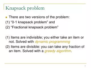
Unidimensional Knapsack Problem m = 1 • Bi-Dimensional Knapsack Problem m = 2 • Quadratic • Hyperbolic • Min-Max • Multi-Objectives • Bi-Level • Cardinality • Multiple-choice • Precedence • Demand • Quadratic Variants of Knapsack Problem Objective Constraints
Multidemand Multidimensional Knapsack Problem Knapsack & Covering Problem
Multi-Choice Multidimensional Knapsack Problem • g : Number of groups • gi: Number of items in group i • cij : Profit associated to item j of group i • : Consuming resource k by item j of group i • bk: Capacity of resource k
Multidimensional Knapsack Problem with Generalized Upper Bound constraints
Knapsack Constrained Maximum Spanning Tree Problem Aggarwal et al (1982) KCMST problem arises in practice in situations where the aim is to design a mobile communication network under a strict limit on total costs.
Generalized Knapsack Problem Suzuki (1978)
Disjunctively Constrained Knapsack Problem Yamada et al (2002)
Max Min Multidimensional Knapsack Problem Introduction to minimax, Demyanov Molozemov 1974 Minimax and applications, Du, Pardalos 1995 Robust optimization applications, Yu 1996 A virtual pegging approach, Taniguchi, Yamada, Kataoka 2009 Iterative Heuristics, Mansi, Hanafi, Wilbaut 2009
Knapsack Sharing Problem Brown (1979)
Bilevel Knapsack Problem Leader objective function (BKP) Follower objective function Follower problem Moore, Bard 1990 => B2 = 0 Dempe, Richter 2000 Hanafi, Mansi, Brotcorne 2009 15
Tabu Search & Dynamic Programming • Metaheuristic: Tabu Search (TS) • Very powerful method on many optimization problems • Based on the exploration of a neighbourhood • Exact method: Dynamic Programming (DP) • Efficient for small-sized problem • Can be used for solving a series of "similar" problem • Can be enhanced by adding reduction rules
Tabu Search & Dynamic Programming |N|= 8 N1 Partition N2 Dynamic Programming with Fixation on N1 Recurrence Tabu Search on N2 • |N 1| small and depends on the instance and the machine. • How defining N 1 and N 2 ?
Dynamic Programming (Bellman, 1957) • Recurrence relation for the MKP • In our case all the subproblems concern the same variables and only g varies
Reduction Rules • Let x0 be a feasible solution of the MKP. Order the variables such that: • Proposition 1 (Optimality): Let , • Proposition 2 (Fixation): Balev, Fréville, Yanev and Andonov, 2001.
Dynamic Programming as a Heuristic N 1 P Initial solution:x0 N 2 Order the variables: uj upper bound of P(e-x0,{j}) n, m Partition the set of variables: N 1 and N 2 if cx1 > cx0 or if |F| > 0 the machine List L (with all the optimal values) Fixation F x1 Dynamic Programming
Global Intensification (GI) Mechanism Dynamic Programming List L (with all the optimal values) Fixation F x1 Tabu Search: performed on N 2 and uses L x* If cx* > cx1 then restart the algorithm with x* as the initial solution
N 1 1 0 1 0 1 0 1 0 N 2 ? 0 1 ? ? 1 1 0 Tabu Search • TS on N2 (|N2| = n2) • Neighbourhood of the current solution x2 on N2: • Evaluation of a solution over N from a solution over N2 Scan in L
Computational Environment • Algorithm coded in C language • The results have been obtained on a Solaris Ultra Sparc workstation 300MHz • n1 15% of n • OR-Library : 270 correlated instances • n = 100, 250, 500 and m = 5, 10, 30 • 30 instances for each (n,m)
A Summary of the Results Each value = average over 30 instances %: average gap wrt CPLEX (with the same computational time) CPU: in seconds TS alone: Tabu Search algorithm without global intensification mechanism
Relaxation Definition : Let (P) max{ f(x) : xX} (R) max{ g(x) : xY} Problem R is a relaxation of P if 1) XY 2) xX : f(x) ≤g(x). Properties - v(P) ≤ v(R) - Let x* an optimal solution of R, if x* is feasible for P and f(x*)=g(x*) then x* is an optimal solution of P
LP-Relaxation Dantzig (1957) max cx (LP) s.t. Ax ≤ b x [0, 1]n Properties : - v(MKP) ≤ v(LP) - Let x* an optimal solution of LP, if x* {0,1}n then x* is an optimal solution of MKP
MIP Relaxation Hanafi & Wilbaut (06), Glover (06) • Let x0 {0, 1}n and J N • Remarks: • MIP(x0,) = LP(P),MIP(x0,N) = P • v(MIP(x0,J)) v(MIP(x0,J’) if J J’ • Stronger bound : v(P) v(MIP(P,J)) v(LP(P))
Lagrangean Relaxation Held & Krap (71), Geoffrion (74) • Lagrangean Relaxation : 0 LR() max{cx + (b – Ax) : xX} • Lagrangean Dual : (L) min{v(LR()) : 0} Properties : - v(MKP) ≤ v(L) ≤v(LR()) - Let x* be an optimal solution of LR(*), if *(b – Ax*)= 0 and x* is feasible for P then x* is an optimal solution of P
cx LP LR P Conv GeometricInterpretation :v(L) = max{cx : Ax≤ b, x co(X)}
Lagrangean Decomposition Guignard & Kim (87)
Lagrangean Decomposition Sub-problem 2 Sub-problem 1
cx LP LR LD P Conv Conv Geometric Interpretation Sub Pb 2 Sub Pb 1
Surrogate Relaxation Glover (65) • Relaxation surrogate : 0 SR() max{cx : Ax ≤b, x X} Dual surrogate corresponding : (S) min{v(SR()) : 0}. Propriétés : - v(MKP) ≤ v(S) ≤v(SR()) - Let x* be an optimal solution of SR(), if x* is feasible for MKP then x* is an optimal solution of MKP • (S) min{v(SR()) : U = { 0: |||| = 1}}
CompositeRelaxation Greenberg & Pierskalla (70) • Composite Relaxation : , ≥ 0 CR(, ) max{cx + (b – Ax) : Ax≤b and xX} Composite Dual : (C) min{v(CR(, )) : , ≥ 0} Remarks : - v(LR()) = v(CR(, 0)) - v(SR()) = v(CR(0, ))
Comparisons v(P) v(C) v(S) v(L) v(LP)
Properties of Relaxation Functions • Lagrangean function v(LR()) is convex and piecewise-linear if X is finite • Surrogate function surrogate v(SR()) is quasi-convex and piecewise-linear if X is finite • Composite function v(CR(, )) is non convex, non quasi-convex
Methods for Dual • (Quasi-)Sub-gradient : ’ = + t g g : sub-gradient of f( )=v(R()) t : Stepwise x*() an optimal solution of R() g() = b – Ax*() a sub-gradient of f() • Bundle method, linearization, etc.
1 2 max * 0 Intersection Algorithm Fisher (75), Yu (90), Hanafi (98) v(LR())
A1x≤b1 x*(u) A2x≤b2 uAx≤ub Extended Dichotomy Algorithmfor Bi-dimensional Knapsack Fréville & Plateau (93), Hanafi (93)
Relaxation-based Heuristics • u = u°, UB = g(u), LB = f(x0) • Repeat • let x*(u) an optimal of the current relaxation R(u) • let x(u) the projection of x*(u) an the feasible set of P • UB = min(UB, v(R(u))) • LB = max(LB, f(x(u))) • Update the current multiplier u
Relaxation-based Heuristics Hanafi & Wilbaut (2006) • Step 1:Solve one or more relaxations of the current problem P to generate one or more constraints. • Step 2:Solve one or more reduced problems induced by the optimal solution(s) of the previous relaxation(s) to obtain one or more feasible solution(s) of the initial problem. • Step 3:If a stopping criteria is satisfied then return the best lower bound. Else add a generated constraint(s) to the problem P and return to step 1.
Space Search • Binary Solution : x {0, 1}n • Improved Heuristic • Continuous Solution : x [0, 1]n • LP-Relaxation • Partial Solution : x {0, 1, *}n where * = free • Branch&Bound, Dynamic Programming, Heuristic • Feasible and Infeasible Solutions • Oscillation, Resolution Search, Dynamic B&B
Reduced Problem • Let x0 {0, 1}n and J N P(x0, J) = (P| xJ = x0J) • Remarks : • P(x0,) = P, v(P(x0,J)) v(P(x0,J’) if J J’ • xJ = x0J(eJ – 2 x0J)xJ+ eJ x0J = 0 • |J| = 1 If v(P(e - x0,{j})) ≤cx0 then x*j = x0j , x*an optimal solution
LP-based Heuristic • Step 1: Solve the LP-relaxation of P to obtain an optimal solution xLP • Step 2: Solve the reduced problem P(xLP,J(xLP)) to generate an optimal solution x0 where J (x) = {jN : xj {0, 1}} • Remarks: • cx0≤ v(P) ≤ cxLP • Relaxation induced neighbourhoods search, Danna et al., 2003 P((xLP+x*)/2,J((xLP+x*))/2) with cx > cx* where x* the best feasible solution
Pseudo-Cut Let y be a vector in {0, 1}n, the following inequality (*) cuts off the solution y without cutting off any other solution in {0, 1}n (*) where J0(x) = {jN : xj= 0} J1(x) = {j N : xj= 1}. Example: (*) is called canonical cut inBalas and Jeroslow,1972.
Partial Pseudo cuts Let x’ be a partial solution in {0, 1, *}n, the inequality dJ(x, x’) = (eJ – 2 x’J)xJ + eJ x’J 1 (*) cuts off x’ and all partial solution dominated by x’. J = {jN: x’j {0,1}}, xJ = (xj : jJ) Remarks : • (*) is called • Pseudo Cut by Glover, 2005. • Canonical Cut by Balas & Jeroslow, 1972, if J = N • dN (x, x’) = Hamming distance over {0, 1}n
Iterative LP-based heuristic (ILPH) Let x* a feasible solution of P v* = cx*; Q = P ; stop = False; while (stop = False) do Let xLP be an optimal solution of LP(Q); J = J(xLP); Let x0 be an optimal solution of (Q|(eJ – 2xLPJ)xJk – eJxLPJ) if cx0> v* then x* = x0; v* = cx0 Q = (Q | (eJ – 2xLPJ)xJk + 1 – eJxLPJ) if cxLP-v* < 1 then stop = True end while
Theorem : Finite Convergence The algorithm ILPH converges to an optimal solution of the problem in a finite number of iterations( 3n). Proof : • v(P) = max(v(P|dxd0), v(P|dxd0 + 1)) • d = (eJ – 2xLPJ, 0) and d0= – eJxLPJ • Number of partial solutions = |{0, 1, *}n|=3n
Convergence of IPLH F(x): set of fractional variables of solution x CPU 400sec (Cplex 10sec) Replace the optimal condition by a total number of iterations