Pro Forma Analysis
Pro Forma Analysis. Agribusiness Finance LESE 306 Fall 2009. PRESENT. PAST. FUTURE. Historical analysis Comparative analysis Historical price and yield trends. Pro forma analysis Forming expectations about future prices, costs and productivity Ad hoc extrapolations

Pro Forma Analysis
E N D
Presentation Transcript
Pro Forma Analysis Agribusiness FinanceLESE 306 Fall 2009
PRESENT PAST FUTURE • Historical analysis • Comparative analysis • Historical price and yield trends • Pro forma analysis • Forming expectations about future prices, costs and productivity • Ad hoc extrapolations • Projections based upon available outlook data • Projections based upon econometric analysis
Timeline Required for Capital Budgeting… Assume it is the year 2009 and John Deere wants to project farm machinery and equipment sales over the next six years to determine if plant expansion is necessary. 2009 2010 2011 2012 2013 2014 2015
Timeline Required for Capital Budgeting… Assume it is the year 2009 and John Deere wants to project farm machinery and equipment sales over the next six years to determine if plant expansion is necessary. 2009 2010 2011 2012 2013 2014 2015 Capital budgeting models of investment decisions require projections of the annual revenue and cost values over the entire 2010 to 2015 time period.
Ad Hoc Modeling Approaches • Naïve model – using last year’s prices, costs and yields • Simple linear trend extrapolation of historical prices, costs and yields • Using assumptions made by others
Econometric Model Approach • Capturing future supply/demand impacts on prices and unit costs • Linkages to commodity policy • Linkages to domestic economy • Linkages to the global economy
Econometric Analysis Based on Time Trend Extrapolation It = f(Yeart)
A linear time trend projection of future farm machinery and equipment sales therefore does a poor job of predicting future sales activity.
Econometric Analysis Based on Investment Theory It = f{[E(Pt)×E(Qt)]/E(ct)}
An econometric model based on investment theory does a muchbetter job of predicting future sales activity.
Concept of Derived Demand for Farm Machinery The demand for farm machinery is driven by the expected net economic benefit from use of the machine….
D D S S Crop Market Equilibrium Price S D • Supply consists of: • Beginning stocks • Production • Imports Pe • Demand consists of: • Industrial use • Feed use • Exports • Ending stocks Quantity Qe
Forecasting Future Commodity Price Trends D $7 S D = a – bP + cYD + eX $4 Own price Other factors Disposable income $1 10
Forecasting Future Commodity Price Trends D $7 S Own price Input costs Other factors $4 S = n + mP – rC + sZ $1 10
Projecting Commodity Price D $7 S D = 10 – 6P + .3YD + 1.2X D = S $4 S = 2 + 4P – .2C + 1.02Z $1 10 Substitute the demand and supply equations into the the equilibrium condition and solve for price
Point Forecast Assumptions Assumes perfect knowledge of outcomes in all 5 areas!!!! PE QE
Structural Pro Forma Analysis Supply-side risk for a given price… PE QLQEQH
Structural Pro Forma Analysis Demand and supply-side risk and potential price variability… PH PE PL QLQEQH
Econometric Analysis – Food Use Own price elasticity Income elasticity Cross price elasticity
Observed and Predicted Values For Wheat Food Use
Remaining Steps to Forecasting the Price of Commodity • Develop similar econometric equations for feed use, exports and ending stock demand. • Develop econometric equations for production and import supply. • Substitute the estimated equations into the market equilibrium definition (QD=QS) and solve for the price where excess demand equals zero.
The Market Model Demand equations: Qd,i = a0 - a1(Price) + ai (demand shifters) Supply equation: Qs,i = b0 +b1(price) + bi (supply shifters) Market equilibrium: ΣQd,i = ΣQs,i
Conclusions • Econometric models preferred over naïve models and linear time trend models. • Much more accurate. • Provide much more information (e.g., elasticities). • Allow for sensitivity analysis with independent (exogenous) variables when evaluating potential variability about expected trends.