Download
1 / 30
310 likes | 548 Vues
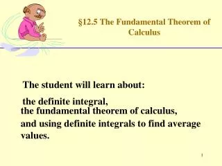
§12.5 The Fundamental Theorem of Calculus. The student will learn about:. the definite integral,. the fundamental theorem of calculus,. and using definite integrals to find average values. §13.1 Area Between Curves. The student will learn about:. Area between a curve and the x axis ,.

E N D
§12.5 The Fundamental Theorem of Calculus The student will learn about: the definite integral, the fundamental theorem of calculus, and using definite integrals to find average values.
§13.1 Area Between Curves The student will learn about: Area between a curve and the x axis , area between two curves, and an application.
Negative Values If f (x) is positive for some values of x on [a,b] and negative for others, then the definite integral symbol Represents the cumulative sum of the signed areas between the graph of f (x) and the x axis where areas above are positive and areas below are counted negatively. Represents the cumulative sum of the signed areas between the graph of f (x) and the x axis where areas above are positive and areas below are counted negatively. Remember area measure is never negative! y = f (x) B a A b
Negative Values The area between the graph of a negative function and the x axis is equal to the definite integral of the negative of the function. y = f (x) B a A b c
Area Between Curve and x axis The area between f (x) and the x axis can be found as follows: For f (x) 0 over [a, b]: Area = i.e. f (x ) is above the x axis. For f (x) 0 over [a, b]: Area = i.e. f (x ) is below the x axis.
A 1 A 2 Example Find the area bounded by y = 4 – x 2; y = 0, 1 x 4. Area = A 1 - A 2 = 8 – 8/3 – (16 – 64/3 – 8 + 8/3) = 16
Area Between Two Curves Theorem 1. If f (x) g (x) over the interval [a, b], then the area bounded by y = f (x) and y = g (x) for a x b is given by: f (x) A g (x) a b
= 3x – x 3 /3 + x = Example Find the area bounded by y = x 2 - 1; y = 3. Note the two curves intersect at –2 and 2 and y = 3 is the larger function on –2 x 2. 6 – 8/3 + 2 – (-6 + 8/3 – 2)
Example Find the area bounded by y = x 2 - 1; y = 3. Note many graphing calculators have numeric integration routines. = 10.667
Income Distribution - Application The U.S. Bureau of the Census compiles data on distribution of income among families. This data can be fitted to a curve using regression analysis. This curve is called a Lorenz curve. The variable x represents the cumulative percentage of families at or below the given income level. The variable y represents the cumulative percentage of total family income received. Absolute equality of income would occur if the area between the Lorenz curve and y = x were 0. The maximum possible area between the Lorenz curve and y = x is ½ the area of the triangle below y = x indicating absolute inequality of income (i.e. one family has all the income).
Gini index of Income Concentration If y = f (x) is the Lorenz curve, then Index of income concentration = Income Distribution - Application The ratio of the area bounded by y = x and the Lorenz curve is the area of the triangle under the line y = x form x = 0 to x = 1 is called the index of income concentration. A measure of 0 indicates absolute equality. A measure of 1 indicates absolute inequality.
Example A country is planning changes in tax structure in order to provide a more equitable distribution of income. The two Lorenz curves are: f (x) = x 2.3 currently and g (x) = 0.4x + 0.6x 2 proposed. Will the proposed changes work? Currently: Gini index of income concentration = 0.3939 Future: Gini index of income concentration = 0.20
Summary. We reviewed the definite integral as the area between a curve and the x axis. We learned how to calculate area when the curve was below the x axis. We learned how to calculate the area between two curves. We learned about the Lorenz curve and the Gini index of income concentration.
Practice Problems §7.1; 1, 3, 7, 11, 15, 17, 21, 27, 31, 35, 39, 43, 47, 51, 55, 59, 61, 65, 69, 75, 77.
§13.2 Applications The student will learn about: Probability density functions , Continuous income stream, Future value of a continuous income stream, and Consumers’ and producers’ surplus.
A probability density function must satisfy: 1. f (x) 0 for all x 3. If [c, d] is a subinterval then Probability (c x d) = Probability Density Function 2. The area under the graph of f (x) = 1 Probability density function
Probability (3 x 6) = = Example In a certain city the daily use of water in hundreds of gallons per household is a continuous random variable with probability density function Find the probability that a household chosen at random will use between 300 and 600 gallons. = - e – . 9 + e - . 45 .23
Total income = a Total Income b Continuous Income Stream Total Income for a Continuous Income Stream. If f (t) is the rate of flow of a continuous income stream, the total income produced during the time period from t = a to t = b is:
Total income = = 10,000 e 0.06 t Example Find the total income produced by a continuous income stream in the first 2 years if the rate of flow is f (t) = 600 e 0.06 t = 10,000 (e 0.12 – 1) $1,275
Future Valueof a Continuous Income Stream From the previous example and previous work we are familiar with the continuous compound interest formula A = Pert. Future Value of a Continuous Income Stream If f (t) is the rate of flow of a continuous income stream, 0 t T, and if the income is continuously invested at a rate r compounded continuously, the the future value, FV, at the end of T years is given by
Example Let’s continue the previous example where f (t) = 600 e 0.06 t Find the Future Value in 2 years at a rate of 10%. r = 0.10, T = 2, f (t) = 600 e 0.06t = (600) (1.22140) (1.92209) = 1,408.59
If (x, p) is a point on the graph of the price-demand equation p = D (x), then the consumers’ surplus, CS, at a price level of p is Which is the area between p = p and p = D (x) from x = 0 to x = x. The consumers’ surplus represents the total savings to consumers who are willing to pay more than p for the product but are still able to buy the product for p. CS x p Consumers’ Surplus
Step 1. Find x, the demand when the price is p = 120: p = 200 – 0.02x 120 = 200 – 0.02x x = 4000 Example Find the consumers’ surplus at a price level of p = $120 for the price-demand equation p = D (x) = 200 – 0.02x
x = 4000 = 80x – 0.01x 2 Example - continued Find the consumers’ surplus at a price level of p = $120 for the price-demand equation p = D (x) = 200 – 0.02x Step 2. Find the consumers’ surplus: = 320,000 – 160,000 = = 320,000 – 160,000 = $160,000
If (x, p) is a point on the graph of the price-supply equation p = S (x), then the producers’ surplus, PS, at a price level of p is which is the area between p = p and p = S (x) from x = 0 to x = x. The producers’ surplus represents the total gain to producers who are willing to supply units at a lower price than p but are still able to supply units at p. CS x p Producers’’ Surplus
Step 1. Find x, the supply when the price is p = 55: p = 15 + 0.1 x + 0.003 x 2 55 = 15 + 0.1 x + 0.003 x 2 0 = 0.003 x 2 +0.1 x - 40 Solving for x using a graphing utility. x = 100 Example Find the producers’ surplus at a price level of p = $55 for the price-supply equation p = S (x) = 15 + 0.1 x + 0.003 x 2
= 40x – 0.05x 2 – 0.001 x 3 x = 100 Example - continued Find the producers’ surplus at a price level of p = $55 for the price-supply equation p = S (x) = 15 + 0.1 x + 0.003 x 2 Step 2. Find the producers’ surplus: = 4,000 – 500 – 1,000 = = 4,000 – 500 – 1,000 = $2,500
Summary. We learned how to use a probability density function. We defined and used a continuous income stream. We found the future value of a continuous income stream. We defined and calculated a consumer’s surplus. We defined and calculated a producer’s surplus.
Practice Problems §7.2; 1, 3, 5, 7, 9, 13, 17, 21, 29, 33, 37, 41, 43, 47, 51.