Viscosity
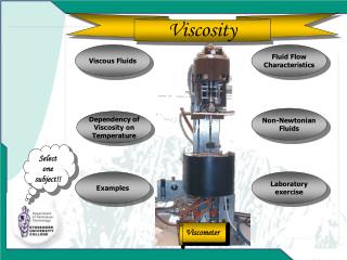
Viscosity. Fluid Flow Characteristics. Viscous Fluids. Dependency of Viscosity on Temperature. Non-Newtonian Fluids. Select one subject!!. Laboratory exercise. Examples. Viscometer. Select one subject. Section 1: Viscous Fluids. Horizontal flow of viscous fluids.

Viscosity
E N D
Presentation Transcript
Viscosity Fluid Flow Characteristics Viscous Fluids Dependency of Viscosity on Temperature Non-NewtonianFluids Select one subject!! Laboratory exercise Examples Viscometer
Select one subject Section 1: Viscous Fluids Horizontal flow of viscous fluids Continuity equation for viscous flow Viscous flow through a porous medium made up of a bundle of identical tubes Viscous flow in a cylindrical tube Exercise: capillary tube viscosity measurement Back Next
Two large parallel plates of area A Y t < 0 y t = 0 x V t is small V t is large V Horizontal flow of Viscous Fluids Lower plate is set in motion with constant velocity The fluid start to move due to motion of the plate After a while the fluid enter a steady state velocity profile Y – a very small distance To maintain this steady state motion, a constant force F is required Back Next
The force F per unit area A is proportional to the velocity V in the distance Y; the constant of proportionally is called the viscosity of the fluid. The force may be expressed: Back Next
Also used is the so called Newton`s equation of viscosity: The shear stress The fluid velocity in x- direction The fluid viscosity The dimensions: And By definition: Explicit: Back Next
Typical values of viscosity of some fluids: Temperature Celsius Viscosity Castor Oil, Poise[p] Viscosity Water, centiPoise[cp] Viscosity Air, Micro Poise[ p] 0 53,00 1,792 171 20 9,86 1,005 181 40 2,31 0,656 190 60 0,80 0,469 200 80 0,30 0,357 209 100 0,17 0,284 218 Back Next
y y X Continuity equation for viscous flow The flow will have the biggest velocity at the top (the surface ) A liquid is flowing in a open channel Fluid flows in an open channel The flow velocity will approximately be zero at the bottom, due to retardation when liquid molecules colliding with the non-moving bottom A graphic presentation of this phenomena is shown here Back Next
Jp – is often characterised as the momentum intensity or as the shear stress, The unit : Transferred momentum pr. time pr. area The change in fluid flow velocity pr. distance between the two layers Viscosity is here defined as s proportionality constant, similar to what was done in the case of defining absolute permeability Back Next
y S` x S z The change of momentum intensity the box: dy is the width of the box and S = S` is the cross-section Momentum transfer between layers S and S` in Newtonian viscous flow Back Next
The momentum density inside the box is defined by . The change of momentum pr. time inside the box is : is the sum of all forces acting on the box. Let f symbolise a force of more general origin. Combining with the equation from last page gives us: Substituting: Back Next
s` s r r + dr R Viscous flow in a cylindrical tube To develop the continuity equation for this example, dr (a thin layer), of liquid is considered at a radius r. Cross-section of viscous flow through a cylindrical tube Viscous flow in a tube is characterised by a radial decreasing flow velocity, because of the boundary effect of the tube wall Back Next
Here the flux area S is varying and . Defining the change in the momentum density inside the cylindrical volume, as , the general equation for laminar flow is: The momentum flux through the cylindrical volume: The momentum intensity jp is redefined according to the geometric conditions in this example: The minus sign show that the flow velocity vx is decreasing when the radius r is increasing Back Next
At a constant pressure drop along the tube, no velocity variation is observed . The continuity equation for viscous flow in a cylindrical tube is: This is under stationary conditions. Back Next
Since the maximum flow velocity, vx(r=0) in the centre of the tube is less then infinity; C1=0 • Since the flow velocity is zero along the tube wall; vx(r=R)=0 and The general solution of the previous equation, found by integrating twice, is: The general constants are found by considering the boundary conditions. For this example the flow is directed along the x-axis The solution is then: Back Next
If the outer force, driving the liquid through the tube is the pressure drop along a tube length then and: R -R Velocity profile in cylindrical tube flow Defines a the laminar viscous flow pattern This flow velocity profile in the tube is given by the formula above. Back Next
Viscous flow through a porous medium made up of a bundle of identical tubes The incremental flow rate through a fraction of the cross-section of a capillary tube can be expressed: The total flow rate can be found by integration: For the sake of convenience we may present the last equation in the following form: This is also known as the Poiseuille`s equation, where A is the cross-section of the capillary tube Back Next
Where is the capillary tube cross-section and A is the cross-section of the porous medium. From the equation above the permeability of the medium where capillary tubes are packed together is found: Where the porosity of the bundle of capillary tubes is given by: Considering a porous medium as a bundle of identical capillary tubes, the total flow qp through the medium is: Back Next
2R Exercise: Capillary tube viscosity measurement Fluid viscosity may also be estimated by the measuring the volume of fluid flowing through a capillary tube pr. time (as the figure below). Rewriting the Poiseuille`s equation an expression for the dynamic fluid viscosity is written: Back Next
For horizontal flow through a capillary tube of length and radius R, the time it takes to fill a certain volume is measured. The flow pressure , is fixed during the process, by maintaining a constant fluid level at a certain elevation above the capillary tube. The accuracy in these measurements is strongly related to the fabrication accuracy of the capillary tubes, as can be seen from the formula above. If the relative uncertainty is considered, Which means that if the relative accuracy in the tube-radius is +/- 2-3 %, then the relative accuracy in the viscosity is about +/- 10 %. A small variation in capillary tube fabrication induces large uncertainty in the viscosity measurement. Back Next
Section 2: Fluid Flow Characteristics For laminar flow in a cylindrical tube we have derived Poiseuille`s equation: For turbulent flow in a cylindrical tube, an empirical law, called Fanning`s equation has been found: This factor is dependent of the tube surface roughness, but also on the flow regime established in the tube F – the Fanning friction factor Back Next
The flow regime is correlated to the Reynolds number, which characterises the fluid flow in the tube. The Reynolds number, Re, is defined as a dimensionless number balancing the turbulent and the viscous (laminar) flow [ ]. v – the average flow velocity – density – the fluid viscosity 2R is the spatial dimension where the flow occur – the diameter of a capillary tube or width of an open channel. From experimental studies an upper limit for laminar flow has been defined at a Reynolds number; Re =2000. Above this number, turbulent flow will dominate. (This limit is not absolute and may therefore change somewhat depending on the experimental conditions.) Back Next
In the case of porous flow, the velocity v in the previous equation should be the pore flow velocity, where and R is the pore radius. The Reynolds number for flow in a porous medium is: Typical parameters for laboratory liquid flow experiments: - the bulk velocity pore dimension bulk velocity fluid density porosity viscosity residual oil saturation Back Next
In case of reservoir flow, the ”normal” reservoir flow velocity is ca. 1 foot/day or , which indicate that turbulent liquid flow under reservoir conditions is not very likely to occur. Using the previous table we find Reynolds number Re = 1 (ca.), for laboratory core flow, which is far below the limit of turbulent flow. For gas, turbulent flow may occur if the potentials are steep enough. If the formula for Reynolds number and Poiseuille`s law is compared: The only fluid dependent parameters are the density and the viscosity Comparing the Reynolds number for typical values of gas and oil : Demonstrates the possibilities for turbulent when gas is flowing in a porous medium Back Next
Heavy oil Viscosity, cp Light oil Temperature, K Section 3: Dependency of Viscosity on Temperature The Viscosity of liquids decreases with increasing temperature. For gas it`s the opposite; viscosity increase with increasing temperature. Back Next
Temperature depending viscosity of gases expressed by the Satterland`s equation: Where K and C are constants depending on the type of gas. Another commonly equation: Where n depends on the type of gas (1 < n < 0,75) Back Next
Here is the breaking shear stress • is the so-called structural viscosity there is no fluid flow Section 4: Non-Newtonian Fluids Viscous-Plastic fluids Bingham (1916) and Shvedov (1889) investigated the rheology of viscous-plastic fluids. These fluids also feature elasticity in addition to viscosity. Equation describing viscous-plastic fluids: Some oils, drilling mud and cements slurries represent viscous-plastic fluids. Back Next
Pseudo-Plastic fluids Some fluids do not have breaking shear stress but rather, their apparent viscosity depends on a shear rate: Which means that their apparent viscosity decreases when dv/dy grows: Back Next
Section 5: Examples 6.2.1 Water viscosity at reservoir conditions 6.2.2 Falling sphere viscosity measurement 6.2.4 Rotating cylinder viscosity measurement Back Next
Water viscosity is primarily a function of temperature. Salinity has also a slight influence on . The pure water viscosity is listed in viscous fluids section. Due to correction foe salinity and reservoir temperature, the normal range of viscosity at reservoir conditions is from 0,2 to 1,0 cP. At a res. temp. of , the water viscosity will be: NB! Even if the temperature is above , water at reservoir condition will still be in a liquid phase since the res. Pressure is quite high as compared to surface condition. Water viscosity at reservoir conditions Correlation for estimation of water viscosity at res. temp. : Water viscosity is measured in cP and temperature in Fahrenheit Back Next
The force Fs is given by Stoke`s law: – density of the metal sphere – density of the fluid h r – sphere radius Vs – thermal speed – viscosity Falling sphere viscosity measurement A metal sphere falling in viscous fluid reaches a constant velocity vs Then the viscous retarding force plus the buoyancy force equals the weight of the sphere The weight of the sphere will balance the viscous force plus the buoyancy force at the terminal sphere velocity when the sum of forces acting on the sphere is zero g – the constant of gravitation Back Next
Viscosity can be estimated by measuring the falling speed of the metal sphere in a cylindrical tube: ( ) Alternatively; measuring the time : C – characteristic constant, determined through calibration with a fluid of known viscosity Back Next
h The outer cylinder: – Radius Held stationary by a spring balance which measures the torque M The inner cylinder: – Radius – Constant Angular velocity M Rotating cylinder viscosity measurement Here we will also Look at the motion of a fluid between two coaxial cylinders Due to the elastic force (in the fluid) a viscosity shear will exist there One cylinder is rotating with an angular velocity The other one is kept constant h – the fluid height level on the two cylinders Back Next
For a certain viscometer, the viscosity as function of angular momentum and angular velocity is: C – the characteristic constant for the viscometer Back Next
Section 6: Laboratory exercise Back Next
Section 6: Back Next