Acceleration Methods for Numerical Solution of the Boltzmann Equation
360 likes | 561 Vues
Acceleration Methods for Numerical Solution of the Boltzmann Equation. Husain Al-Mohssen. Motivation & Introduction Problem Statement Proposed Approach Important Implementation Details Examples Discussion Future Work. Outline. Motivation.

Acceleration Methods for Numerical Solution of the Boltzmann Equation
E N D
Presentation Transcript
Acceleration Methods for Numerical Solution of the Boltzmann Equation Husain Al-Mohssen
Motivation & Introduction Problem Statement Proposed Approach Important Implementation Details Examples Discussion Future Work Outline
Motivation • Nano-Micro devices have been developed recently with very small dimensions: • DLP (Length) • HD read/write head (Gap Length) • At STP an air molecule travels an average distance between collisions • As may be expected the Navier-Stokes (NS) description of the flow starts to break down as system length becomes comparable to l • Accurate engineering models are essential for the understanding and design of such systems
Motivation (cnt) • The Knudsen number is defined as the ratio of the mean free path to a characteristic dimension (Kn= l/L). Kn is a measure of the degree of departure from the NS description • Kn Regimes: • Recent applications are at low Ma number
Introduction (cnt) The Boltzmann Equation (BE) in normalized form: • Follows from the dilute gas assumption • Valid for all Kn • 7D(1time+3Space+3Velocity) nonlinear Integro-differential equation
Introduction (cnt) Numerical Methods of Solving the BE: • Particle based: DSMC • Collisionless advection step + collision steps are successively applied. • Can be shown to simulate BE exactly in the limit of large numbers [Wagner 1992]. • Chronic sampling problems at low speeds [Hadjiconstantinou et al, 2003]. • Low Ma lmit particularly troublesome • Approximations of the BE • Linearized (has many advantages espcially when Ma<<1; still requires numcerical solution) • BGK CI Replaced with • Numerical solutions of the BE • Recently Baker and Hadjiconstantinou (B&H) proposed a method to solve the BE at low Ma in a relatively efficient manner.
Proposed Solution Methodology F(ui) and F’(ui) F(u) x ui+1 ui
Simplified Flow Chart of Method Start Find Estimate Integrate BE to find Use Broyden to find from and Find Converged? No Yes End
1D Graphical Analog F[u] u
Important Implementation Details (BE Portions) Shift f to target mean Integrate BE 1 2 3
Step1: Equilibrate f Step2: Sample Calculation to find Flow Chart of Method Start Find Estimate Integrate BE Use Broyden to find from and Find Converged? No Yes End
U 0.04 Exaggerated Kn Layer 0.02 100 200 300 400 500 Node # -0.02 -0.04 Exaggerated Kn Layer Examples
kn=0.1 0.0015 0.001 0.0005 20 40 60 80 100 120 -0.0005 -0.001 -0.0015 Examples (cnt) Knudsen Layer Broyden Solution Exact layer Convergence History 512 nodes, kn =0.1
The End Questions?
Plot of Convergence Rates of Different Methods • Plot of error for Direct integration, Broyden and Baker Implicit code. Kn=0.025 # of nodes 128. (log[Error] vs. log[CI evaluations])
Error of Broyden vs. noise of F • Show how sig=sig/N_inf in multidimensions
Broyden Step • Broden formula • Formula constraints • Broyden Formula derivation
Backup slides+notes • [[check conv. History 4 high kn and 512]] • “proper” kndsen layer with 100^3 and lower noise kn=0.1 and at least 128 nodes. Replace one already in presentation • Change Conv. History plto to 512 and kn0.025 and 30^3 cells • N_inf vs. Kn for our pb’s to show our rough break point….
DSMC Performance Scaling (Backup) Direct Integration Cost: Broyden Cost: Slope Sampling Scaling is key: Analysis assumes sampling a small portion of run =>
dt .01 , g .1 Red dt .1 g .1 Green dt .1 g90 Blue dt .1 , .01 g1 Orange = = = = 0.0001 0.00001 - 6 1. 10 ´ - 7 1. 10 ´ - 8 1. 10 ´ 10 100 1000 B&H Noise for Different Paramters(Backup) For little extra computational Effort you get a dramatic decrease in measurement error. compare for example pt. A, B and C. A Kn=? If only interested in eng. Accuracy N_inf=10^-4/sig_sample Cost A=Cost B Cost C=10 Cost A B C
Distribution Function initilization (Backup) • Plot of norm f vs. step [[Possibly for multiple kn [[what kn? What state of F?]]
Scaling Arguments (Backup) • Why is it always O(10)? Well possibly because of this: • As per Kelly Newton’s is q-Quadratic and secent is Q-superlinear; Broyden is somewhere in between. • The other plot is the MMA result using [a] x/nnn + noise • Kelly says eps=K eps^2 not exp[-2t] MMA Model Problem in Multi-D with Noise
Can u answer these Questions • Is it possible that O(10) will increase with less noise Requrement • If u reduce Dt sample to decrease noise, don’t u increase N_inf??!!! • [[Re-initializing a Run after it reaches its minimum noise level with less noise as a method of Confirming convergance or reducing noise (NB: since we are somehow finding the null space of the Jacobian aren’t we somehow garanteed to have a sick matrix when we stall?)]]
Can u Explain B&H? • What is importance sampling? & how is it applied to CI? Write the appt. version of CI. • What is control variate M/C interation? • How is the finite volume Spliting method implemented? What are the various Stability conditions?
Integration Stability Codnition • CI step • Convection Step • Implicit step?
-7 -6 -5 -4 Log10[Input Noise] -1 -2 Log10[error] 32 -3 16 512 -4 128 -5 64