KYIV SCHOOL OF ECONOMICS Financial Econometrics (2nd part): Introduction to Financial Time Series

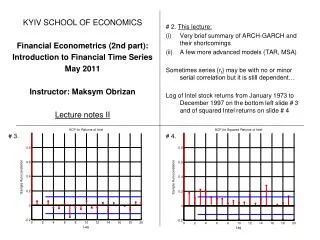
1. KYIV SCHOOL OF ECONOMICS Financial Econometrics (2nd part): Introduction to Financial Time Series May 2011 Instructor: MaksymObrizan Lecture notes II # 2. This lecture: • Very brief summary of ARCH-GARCH and their shortcomings • A few more advanced models (TAR, MSA) Sometimes series {rt} may be with no or minor serial correlation but it is still dependent… Log of Intel stock returns from January 1973 to December 1997 on the bottom left slide # 3 and of squared Intel returns on slide # 4 # 3. # 4.

2. # 5. # 6. Series are uncorrelated but dependent: volatility models attempt to capture such dependence Define shock or mean-corrected return # 7. Then ARCH(m) model assumes In practice, the error term is assumed to follow the standard normal of a standardized Student-t distribution # 8. Practical way of building an ARCH model • Build an ARMA model for the return series to remove any linear dependence in data If the residual series indicates possible ARCH effects – proceed to (ii) and (iii) • Specify the ARCH order and perform estimation (iii) Check the fitted ARCH model for necessary refinements

3. # 9. Fitting an ARCH Model: Model Checking: Obtain standardized shocks Then use Ljung-Box statistic on to check the adequacy of the mean equation and on to check the validity of the volatility equation. Use kurtosis, skewness and QQ-plot of to check if normal distribution is applicable # 10. Shortcomings of ARCH model • Positive and negative shocks have the same effects on volatility • MOTIVATION FOR TAR, MSA MODELS! (ii) ARCH model is restrictive – parameters are constrained by certain intervals for finite moments etc (iii) Sometimes not parsimonious models: use GARCH # 11. GARCH model: Weaknesses of GARCH model are similar to those of ARCH: symmetric response to negative and positive shocks etc # 12. NOTES

4. # 13. Application: daily log returns of IBM stock from July 3, 1962 to December 31, 1999 All the estimates (except the coefficient of rt-2) are highly significant # 14. In addition, the Ljung-Box statistics of the standardized residuals is Q(10) = 11.31 (p-value of 0.33) and of the squared standardized residuals is Q(10) = 11.86 (p-value of 0.29) # 15. The unconditional mean of rt in this model is while in the sample it is only 0.045. What if the model is misspecified? • Motivation for nonlinear models such as TAR and MSA # 16. Threshold Autoregressive (TAR) model

5. # 17. Consider a simple two-regime TAR model # 18. # 19. Observe that this model has coefficient -1.5 However, despite this fact it is stationary and geomertically ergodic if Ergodic theorem – statistical theorem showing that the sample mean of xt converges to the mean of xt # 20. Model behavior depends on xt -1: When it is negative then When it is positive then Question: Which regime will have more observations?

6. # 21. In addition, TAR model has non-zero mean even though the constant terms are zero (think of an AR(m) model with zero constant for a comparison) Re-consider slide # 15 with AR(2)-GARCH(1,1) model of IBM stock: the unconditional mean of 0.065 overpredicted the sample mean of 0.045 Estimate AR(2)-TAR-GARCH(1,1) model and refine it (remove insignificant term in volatility equation) # 22. AR(2)-TAR-GARCH(1,1) of IBM stock # 23. Model fit All coefficients are significant at 5% The unconditional mean? The Ljung-Box statistics applied to standardized residuals does not indicate serial correlations or conditional heteroscedasticity # 24. NOTES:

7. # 25. Convenient to re-write TAR-GARCH(1,1): # 26. Recall the integrated GARCH model (IGARCH is a unit-root GARCH model) For example, IGARCH(1,1) is defined as The unconditional variance of at, and thus of rt, is not defined Meaning: Occasional level shifts in volatility? IGARCH(1,1) with is used in RiskMetrics (Value at Risk calculating) # 27. Thus, under nonpositive deviation the volatility follows an IGARCH(1,1) model without a drift With positive deviation, the volatility has a persistent parameter 0.046+0.885=0.931 which is <1 giving rise to GARCH(1,1) Conclusion: # 28. NOTES:

8. # 29. Markov Switching Model # 30. Application to the US quarterly real GNP # 31. Cont’d # 32. Notes

9. # 33. Nonlinearity tests: Parametric tests The RESET Test for a linear AR(p) model Basic idea: if a linear AR(p) model is adequate then a1 and a2should be zero. # 34. Apply F statistic with g and T-p-g degrees of freedom # 35. Nonlinearity tests: Nonparametric tests Q-statistic of Squared Residuals The null hypothesis of the statistic is # 36. NOTES

10. # 37. Application to the US quarterly civilian unemployment from 1948 to 1993 based on Montgomery, Zarnowitz, Tsay and Tiao (1998) # 38. TAR model # 39. MSA model # 40. NOTES