Download
1 / 35
350 likes | 517 Vues
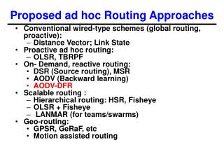
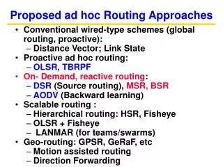
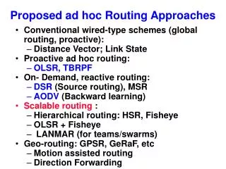
Proposed ad hoc Routing Approaches. Conventional wired-type schemes (global routing, proactive): Distance Vector; Link State Proactive ad hoc routing: OLSR, TBRPF On- Demand, reactive routing: DSR (Source routing), MSR AODV (Backward learning) Scalable routing :

E N D
Proposed ad hoc Routing Approaches • Conventional wired-type schemes (global routing, proactive): • Distance Vector; Link State • Proactive ad hoc routing: • OLSR, TBRPF • On- Demand, reactive routing: • DSR (Source routing), MSR • AODV (Backward learning) • Scalable routing : • Hierarchical routing: HSR, Fisheye • OLSR + Fisheye • LANMAR (for teams/swarms) • Geo-routing: GPSR, GeRaF, etc • Motion assisted routing • Direction Forwarding
Where do we stand? • OLSR and TBRPF can dramatically reduce the “state” sent out on update messages • They are very effective in “dense” networks. • However, the state still grows with O(N) • Neither of the above schemes can handle large scale nets from 10’s to thousands of nodes • What to do?
Hierarchical Routing The previous schemes reduce control traffic O/H but do not significantly reduce routing table size Solution: use hierarchical routing to reduce table size In the process, reduce also control traffic O/H Proposed hierarchical schemes include: • Hierarchical State Routing (HSR) • Fisheye State Routing (FSR) • Landmark Routing • Zone routing (hybrid scheme)
Hierarchical State Routing (HSR) • Loose hierarchical routing in Internet • Main challenge in ad hoc nets: maintain/update the hierarchical partitions in the face of mobility • Solution: distinguish between “physical” partitions and “logical” grouping • physical partitions are based on geographical proximity • logical grouping is based on functional affinity between nodes (e.g., tanks of same battalion, students of same class) • Physical partitions enable reduction of routing overhead • Logical groupings enable efficient location management strategies using Home Agent concepts
3 1 Level = 2 2 3 1 Level = 1 4 2 8 9 6 3 1 Level = 0 10 11 7 5 4 HSR - physical multilevel partitions HSR table at node 5: DestID 1 6 7 <1-2-> <1-4-> <1-3> Path 5-1 5-1-6 5-7 5-1-6 5-7 5-7 HID(5): <1-1-5> HID(6): <3-2-6> Hierarchical addresses (MAC addresses)
HSR - logical partitions and location management • Logical (IP like) type address <subnet,host> • Each subnet corresponds to a particular user group (e.g., tank battalion in the battlefield, search team in a search and rescue operation, etc) • logical subnet spans several physical clusters • Nodes in same subnet tend to have common mobility characteristic (i.e., locality) • logical address is totally distinct from MAC address
HSR - logical partitions and location management (cont’d) • Each subnetwork has at least one Home Agent to manage membership • Each member of the subnet registers its own hierarchical address with Home Agent • periodical/event driven registration; stale addresses are timed out by Home Agent • Home Agent hierarchical addresses propagated via routing tables; or queried at a Name Server • After the source learns the destination’s hierarchical address, it uses it in future packets • Example: Landmark Routing
2 2 2 8 8 8 3 3 3 5 5 5 9 9 9 1 1 1 9 9 9 4 4 4 6 6 6 Hop=1 Hop=1 Hop=1 7 7 7 10 10 10 12 12 12 13 13 13 Hop=2 Hop=2 Hop=2 19 19 19 18 18 18 21 21 21 11 11 11 Hop>2 Hop>2 Hop>2 15 15 15 22 22 22 36 36 36 14 14 14 23 23 23 17 17 17 16 16 16 20 20 20 29 29 29 35 35 35 27 27 27 25 25 25 24 24 24 26 26 26 28 28 28 34 34 34 30 30 30 32 32 32 31 31 31 Fisheye State Routing (FSR) Scope of Fisheye
Fisheye State Routing (FSR) • Topology data base at each node - similar to link state (e.g., OSPF) • Routing information is periodically exchanged with neighbors only ( “Global” State Routing) • similar to distance vector, but exchange entire topology matrix • Routing update frequency decreases with distance to destination • Higher frequency updates within a close zone and lower frequency updates to a remote zone • Highly accurate routing information about the immediate neighborhood of a node; progressively less detail for areas further away from the node
Message Reduction in FSRTC (Topology Control) message LST HOP 0 LST HOP 0:{1} 1:{0,2,3} 2:{5,1,4} 3:{1,4} 4:{5,2,3} 5:{2,4} 1 0 1 1 2 2 0:{1} 1:{0,2,3} 2:{5,1,4} 3:{1,4} 4:{5,2,3} 5:{2,4} 2 1 2 0 1 2 1 3 LST HOP 2 0:{1} 1:{0,2,3} 2:{5,1,4} 3:{1,4} 4:{5,2,3} 5:{2,4} 3 2 1 1 0 1 4 5
Optimized “Fisheye” Link State Routing (OFLSR) • Based on Optimized Link State Routing (OLSR) • Borrows idea from Fisheye State Routing (FSR) • Different frequencies for propagating the Topology Control (TC) message of OLSR to different scopes (e.g. different hops away)
Scalability Property of OFLSR • Scalability to Node Mobility • 100 nodes, 1600mX1600m field, 367m Tx range • IEEE 802.11 radio, 2Mbps channel rate, 10 CBR flows • OLSR confign: hello interval = 1s, TC interval = 2s • OFLSR confign: 4 scopes, each scope is 2 hops except last one Data Packet Delivery Ratio Node mobility speed (m/s) Data Packet Delivery Ratio
Scalability Property of OFLSR • Scalability to Node Mobility Total # of TC relayed Total # of TC received
Scalability Property of OFLSR • Scalability to Network Size • Keep node density, increase # of nodes, no mobility • OLSR confign: hello interval = 2S, TC interval = 4S • OFLSR confign: 4 scopes, each scope is 2 hops except last one Data Packet Delivery Ratio Network Size (# of nodes) Delivery rate vs Network Size
Scalability Property of OFLSR • Scalability to Network Size Total # of TC relayed Total # of TC received
Scalable Ad Hoc Routing using Landmarks and Backbones • The challenge • Tens of thousands of nodes • Nodes move in various patterns • QoS communications requirements • Hostile environment – jamming
Routing • Current MANET solutions have limitations: • (a) proactive routing solutions (eg, Optimal Links State -OLSR) do not scale because of table size and control traffic overhead • (b) on demand routing cannot handle high mobility and dense traffic patterns • (c) explicit hierarchical routing introduces excessive address maintenance O/H in high mobility • MANET protocols do not scale in high mobility • Our approach: • Exploit implicit hierarchy induced by group mobility
Logical Subnet Landmark Solution: Landmark Routing Overlay • Main assumption: nodes move in groups (battlefield) • Groups are predefined or dynamically recognized • Node address: < group ID , Host address> • Landmark elected in each group • Landmarks advertisements maintain the landmark overlay
Logical Subnet Landmark LANMAR Overlay Routing (cont) • Builds upon existing MANET protocols • (1) “local ” routing algorithm that keeps accurate routes within local scope < k hops (e.g., OLSR) • (2) Landmark routes advertised to all mobiles using DSDV • Like Internet: LS + DV
Logical Subnet Landmark LANMAR Overlay Routing (cont) • Packet Forwarding: • A packet to “local” destination is routed directly using local tables • A packet to remote destination is routed to Landmark corresponding to logical addr. • Once the landmark is “in sight”, the direct route to destination is found in local tables • Benefits: low storage, low update traffic O/H
Landmark Routing In action Landmark LM2 LM1 LM3 Logical Subnet dest source local routing Long haul routing • Node address = {subnet ID, Host ID} • Look up local routing table to locate dest fail • Look up landmark table to find destination subnet LM1 • Send a packet toward LM1
Link Overhead of LANMAR • Dramatic O/H reduction from linear to O(N) to O (sqrtN)
LANMAR: Local Scope Optimization • Goal: find local routing scope size that minimizes routing overhead • size of landmark distance vector: O ( N / G) • size of local Link State topology map: O ( m * d ) N: total # of nodes; d: avg # of one-hop neighbors (degree) H (Routing overhead) Total O/H Local route O/H Landmark O/H h (scope size)
LANMAR enhances MANET routing schemes We compare: • MANET routing schemes: DSDV, OLSR and FSR; and (b) same MANET schemes, BUT with LANMAR overlay on top
LANMAR-DSDV LANMAR-FSR OLSR LANMAR-OLSR FSR DSDV Delivery Ratio • DSDV and FSR decrease quickly when number of nodes increases • OLSR generates excessive control packets, cannot exceed 400 nodes
Mobile Backbone Overlay • Landmark Overlay provides routing scalability • However the network is still flat- paths have many hops poor TCP and QoS performance!! • Solution: Mobile Backbone Overlay (MBO) • MBO is a physical overlay – ie long links • MBO provides performance scalability • LANMAR extends “transparently” to the MBO
Landmark UAV Backbone Node Logical Subnet source dest. Landmark routing concept extends transparently to the multilevel backbone Fast BB links are “advertised” and immediately used When BB link fails, the many hop alternate path is chosen
Backbone Network and LANMAR • Why a Backbone “physical” hierarchy? • To improve coverage, scalability and reduce hop delays • Backbone deployment • automatic placement: Relocate backbone nodes from dense to sparse regions (using repulsive forces) • Key result: LANMAR automatically adjusts to Backbone • Combines low routing O/H (LANMARK logical hierarchy) + low hop distance and high bandwidth (Backbone physical hierarchy)
Extending Landmark to Hierarchical Network • Backbone nodes are independently elected • All nodes (including backbone nodes) are running the original LANMAR • In addition, backbone nodes re-broadcast landmark information via higher level links • Backbone Routes preferred by landmark (they are typically shorter)
Extending Landmark (cont) • If backbone node is lost, Landmark routing “fills the gap” while a replacement backbone node is elected • Advantages • Seamless integration of “flat” ad hoc landmark routing with the backbone environment provides instant backup in case of failures • Easy deployment, simple changes to ordinary ground nodes • Remove limitations of strictly hierarchical routing
Variable number of Backbone Nodes • Decrease of average end-to-end delay while increasing # of backbone nodes
Variable number of Backbone Nodes • Increase of delivery fraction while increasing # of backbone nodes
Variable Speed with 1000 nodes Delivery fraction while increasing mobility speed
48 bits 16 bits 64 bits Node ID Network ID GroupID Subnet Mask 11…11 00000000 … 0000000 0000 … 000 LANMAR implementation in IPv6 LINUX environment • Use IPv6’s Group ID to distinguish groups • Support many more members in each group (than IPv4) • A packet to remote destination is routed to corresponding Landmark based on IPv6 address lookup IPv6: