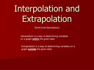
Interpolation and Extrapolation of OBS data Using Interferometry
Interpolation and Extrapolation of OBS data Using Interferometry. Shuqian Dong and Sherif Hanafy. Outlines. Problem Theory Numerical Results Interpolation Extrapolation Summary. Outlines. Problem Theory Numerical Results Interpolation Extrapolation Summary. Problem.

Interpolation and Extrapolation of OBS data Using Interferometry
E N D
Presentation Transcript
Interpolation and Extrapolation of OBS data Using Interferometry Shuqian Dong and Sherif Hanafy
Outlines • Problem • Theory • Numerical Results • Interpolation • Extrapolation • Summary
Outlines • Problem • Theory • Numerical Results • Interpolation • Extrapolation • Summary
Problem • Problem 1: Receiver interval is (sometimes) too big • Solution: Interferometric interpolation • Problem 2: Near offsets are (sometimes) missing • Solution: Interferometric extrapolation
Outlines • Problem • Theory • Numerical Results • Interpolation • Extrapolation • Summary and Future Work
A A A x x x B B B Seabed Seabed Seabed Reflectors Reflectors Theory OBS Single Well Profile OBS G(x|A) Natural Green’s Function Go(x|b)* Model based Green’s Function G(B|A) Interpolated Data
Outlines • Problem • Theory • Numerical Results • Interpolation • Extrapolation • Summary
Field Data Parameters • OBS marine data • A total of 896 shot gather • 179 traces/CSG • Trace interval = 25 m • 2501 samples/trace • 0.004 sec sample interval • Total time = 10 sec
Receiver Gather Sample Number of traces = 401 Trace interval = 25 m Original Data 0.0 Time (s) 10.0 0.0 X (km) 10.0
Outlines • Problem • Theory • Numerical Results • Interpolation • Extrapolation • Summary
Input Data Each 4th trace is used as input Number of input traces = 101 Input trace interval = 100 m Input Data 0.0 Time (s) 10.0 0.0 X (km) 10.0
Output Virtual Receiver Gather Number of output traces = 401 Output trace interval = 25 m Virtual Receiver Gather 0.0 Time (s) 10.0 0.0 X (km) 10.0
Matching Filter • The 101 real traces and the corresponding 101 virtual traces are used to get a correction operator. • Applying this operator on other traces will remove most of the artifacts.
Results after Matching Filter Matching filter is used to suppress the artifacts in the virtual CRG Four Iterations of interpolation and matching filter used to reach this final results Virtual Receiver Gather after Matching Filter 0.0 Time (s) 10.0 0.0 X (km) 10.0
Receiver Gather Sample The original CRG for comparison. Original Data 0.0 Time (s) 10.0 0.0 X (km) 10.0
True vs Virtual Traces Comparisons between true (green-dashed) and virtual (black-solid) traces. Traces used are # 23, 51, 158, 182, 212, 232, 286, 344, 378, and 395
Outlines • Problem • Theory • Numerical Results • Interpolation • Extrapolation • Summary
Extrapolation Theory OBS Single Well Profile OBS A A A x x x B B B Seabed Seabed Seabed Reflectors Reflectors G(x|A) Natural Green’s Function Go(x|b)* Model based Green’s Function G(B|A) Interpolated Data
Input Shot Gather (1st test) 0 Time (s) 3.0 0 250 X (m) 1200
Virtual Shot Gather virtual traces real traces 0 Time (s) 3.0 0 250 X (m) 1200
True Shot Gather 0 Time (s) 3.0 0 X (m) 1200
Input Shot Gather (2nd test) 0 Time (s) 3.0 0 500 1200 X (m)
Virtual Shot Gather virtual traces real traces 0 Time (s) 3.0 0 500 1200 X (m)
True Shot Gather 0 Time (s) 3.0 0 X (m) 1200
Workflow Get Virtual CSG (2) Start Virtual CSG (3) Matching Filter Input Field Data (1) Max. Itr (MF) N Y Find Water Thickness Virtual CSG (4) Generate GF for water multiples Replace virtual traces @ (4) by True traces @ (1) Interpolate/extrapolate missing data Max. Iter N Y Final CSG
Outlines • Problem • Theory • Numerical Results • Interpolation • Extrapolation • Summary
Summary • OBS field data and generated water multiples are used to interferometrically interpolated or extrapolated missing traces • The proposed technique is successfully tested on synthetic and field data • Iteration over interferometric and MF will improve the final results