Download
1 / 32
340 likes | 763 Vues
Ionospheric Scintillations Propagation Model. Y. Béniguel, J-P Adam IEEA, Courbevoie, France. Outline. Overview. Transmitted field calculation. Scattering function calculation (SAR observations). Practical use. Disturbed Ionospheric Regions Affected by Scintillation.

E N D
Ionospheric Scintillations Propagation Model Y. Béniguel, J-P Adam IEEA, Courbevoie, France
Outline • Overview • Transmitted field calculation • Scattering function calculation (SAR observations) • Practical use
Disturbed Ionospheric Regions Affected by Scintillation POLAR CAP PATCHES AURORAL IRREGULARITIES SATCOM GPS PLASMA BUBBLES EQUATORIAL F LAYER ANOMALIES DAY NIGHT MAGNETIC EQUATOR SBR GPS SATCOM
GPS / Galileo signal Receiver level Physical Mechanism Drift velocity
Medium Radar Observations Observations at Kwajalen Islands Courtesy K. Groves, AFRL Observations in Brazil Courtesy E. de Paula, INPE The vertical extent may reach hundreds of kilometers
Development of Inhomogeneities (Modelling) t = 20 s. t = 200 s. Solving momentum and continuity equation small scale model Allows estimating dimensions and temporal behaviour
Signal at receiver level (Measurements) Intensity Phase
Scintillations Parameters S4 and sF S4 and are statistical variables computed over a “reasonable” time period that satisfies both good statistics and stationarity, as follows “Reasonable Time” depends primarily on the effective velocity of the satellite raypath; varies from 10 to 100 seconds; the phase is derived from detrended time series These quantities depend on the density fluctuations in the medium
Seasonal Dependency Seasonal : peak at equinoxes : march & october
Local Time Dependency Local time : post sunset hours
Field received at ground level Solution of the parabolic equation
Field Propagation Equation Solution of the parabolic equation Using the phase index autocorrelation function
Algorithm Phase Screen Technique Propagation : 1st and 3rd terms (Space domain) Diffraction : 1st and 2nd terms (Transform domain)
Phase Screen Technique Transmitter Propagation Scattering Propagation Scattering Propagation Receiver
Medium’s Characterisation 5 days RINEX files in Cayenne considered in the analysis S4 > 0.2 & sigma phi < 2 (filter convergence) 3 parameters :
Anisotropic vs Isotropic LOS B field Additional geometric factor with respect to the 2D case a, b ellipses axes A, B, C trigonometric terms resulting from rotations related to variable changes
How many screens When it converges matched to the electron density profile As many screens as discretisation points along the LOS Current option : one point every 15 km On average : 7 screens
Signal at receiver level Modelling Intensity Phase
Global Maps TEC Map Modelling Scintillation Map Modelling
Comparison with Measurements Upper decile slant S4 index at Marak Parak during September 2000. The dashed line indicates the magnetic equator. GISM Result
Radar Observations Medium Scattering Function
Two Points - Two Frequencies Coherence Function Using the parabolic equation The structure function is quadratic with respect to the distance Same process than previously : propagation 1st & 3rd terms ; diffraction : 1st & 2nd
Propagation 1st & 3rd terms
Medium Scattering Function One screen ; distance = 500 km ; drift velocity = 100 m / s. ; sf = 0.8 F = 400 MHz F = 1.5 GHz The Doppler spreading is related to the drift velocity which can vary with the screen altitude
Including a particular waveform Field intensity Medium’s scattering function
Practical use of the model (GISM)
Medium Characterisation Mean Effects (Sub Models) NeQuick, Terrestrial Magnetic Field (NOAA) Geophysical Parameters SSN, Drift Velocity Scintillations (Fluctuating medium) Spectrum slope (p), BubblesRMS, OuterScale (L0) Anisotropy ratio
Numerical Implementation The model includes an orbit generator (GPS, Glonass, Galileo, …) Inputs Medium Characterisation Geophysical Parameters Scenario Intermediate calculation : LOS,Ionisation along the LOS Outputs Scintillation indices Correlation Distances (Time & Space) Scattering function
Conclusion • The geometry (LOS) with respect to the bubbles orientation is arbitrary • A 1D algorithm applies to all cases • The model allows calculating • the transmitted field at receiver level • the scattering function for radar observations