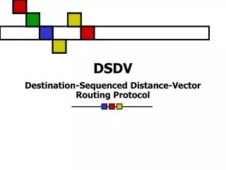
Lecture 2 : The DSDV Protocol
Lecture 2 : The DSDV Protocol. Lecture 2.1 : The Distributed Bellman-Ford Algorithm Lecture 2.2 : The D estination S equenced D istance V ector ( DSDV) protocol. The Routing Problem. S´. D´. S. D.

Lecture 2 : The DSDV Protocol
E N D
Presentation Transcript
Lecture 2 : The DSDV Protocol • Lecture 2.1 : The Distributed Bellman-Ford Algorithm • Lecture 2.2 : The Destination Sequenced Distance Vector (DSDV) protocol Institute for Computer Science, University of Freiburg Western Australian Interactive Virtual Environments Centre (IVEC)
The Routing Problem S´ D´ S D The routing problem is to find a route from S to D when some or all of the nodes are mobile. Institute for Computer Science, University of Freiburg Western Australian Interactive Virtual Environments Centre (IVEC)
Basic Assumptions • We will assume that each node is capable of running fairly complicated algorithms locally. • Each node has the necessary networks layers implemented. In particular, the MAC layer has all the facilities for implementing our protocols. • Our protocols can be implemented using any underlying medium access scheme like TDMA or CSMA. Institute for Computer Science, University of Freiburg Western Australian Interactive Virtual Environments Centre (IVEC)
Nature of Protocols • We will discuss routing protocols for mobile ad hoc networks (MANET). • Routing protocols for MANETs can be classified as either reactive or proactive. • This classification is based on the way a protocol tries to find a route to a destination. Institute for Computer Science, University of Freiburg Western Australian Interactive Virtual Environments Centre (IVEC)
Proactive Protocols • Proactive protocols are based on periodic exchange of control messages and maintaining routing tables. • Each node maintains complete information about the network topology locally. • This information is collected through proactive exchange of partial routing tables stored at each node. Institute for Computer Science, University of Freiburg Western Australian Interactive Virtual Environments Centre (IVEC)
Proactive Protocols • Since each node knows the complete topology, a node can immediately find the best route to a destination. • However, a proactive protocol generates large volume of control messages and this may take up a large part of the available bandwidth. • The control messages may consume almost the entire bandwidth with a large number of nodes and increased mobility. Institute for Computer Science, University of Freiburg Western Australian Interactive Virtual Environments Centre (IVEC)
Reactive Protocols • In a reactive protocol, a route is discovered only when it is necessary. • In other words, the protocol tries to discover a route only on-demand, when it is necessary. • These protocols generate much less control traffic at the cost of latency, i.e., it usually takes more time to find a route compared to a proactive protocol. Institute for Computer Science, University of Freiburg Western Australian Interactive Virtual Environments Centre (IVEC)
Some example protocols • Some examples of proactive protocols are : • Destination Sequenced Distance Vector (DSDV) • STAR • Some examples of reactive protcols are : • Dynamic Source Routing (DSR) • Ad hoc On-demand Distance Vector (AODV) • Temporally Ordered Routing Algorithm (TORA) Institute for Computer Science, University of Freiburg Western Australian Interactive Virtual Environments Centre (IVEC)
Destination Sequenced Distance Vector Protocol • DSDV is a proactive protocol. Each node maintains its own routing table for the entire network. • Consider a node S. Suppose, Sneeds to send a message to node D. • Scan look up the best route to Dfrom its routing table and forward the message to the neighbour along the best route. Institute for Computer Science, University of Freiburg Western Australian Interactive Virtual Environments Centre (IVEC)
DSDV Protocol • The neighbour in turn checks the best route from its own table and forwards the message to its appropriate neighbour. The routing progresses this way. • There are two issues in this protocol : • How to maintain the local routing tables • How to collect enough information for maintaining the local routing tables Institute for Computer Science, University of Freiburg Western Australian Interactive Virtual Environments Centre (IVEC)
Maintaining Local Routing Table • We will first assume that each node has all the necessary information for maintaining its own routing table. • This means that each node knows the complete network as a graph. The information needed is the list of nodes, the edges between the nodes and the cost of each edge. Institute for Computer Science, University of Freiburg Western Australian Interactive Virtual Environments Centre (IVEC)
Maintaining Local Routing Table • Edge costs may involve : distance (number of hops), data rate, price, congestion or delay. • We will assume that the edge cost is 1if two nodes are within the transmission range of each other. • The DSDV protocol can be modified for other edge costs. Institute for Computer Science, University of Freiburg Western Australian Interactive Virtual Environments Centre (IVEC)
How the Local Routing Table is Used • Each node maintains its local routing table by running the distributed Bellman-Ford algorithm. • Each node maintains, for each destination , a set of distances for each neighbour • Node treats neighbour as the next hop for a packet destined for if equals minimum of all Institute for Computer Science, University of Freiburg Western Australian Interactive Virtual Environments Centre (IVEC)
How the local Routing Table is Used 13 k l x i 8 m 23 The message will be sent from i to l as the cost of the path to x is minimum through l Institute for Computer Science, University of Freiburg Western Australian Interactive Virtual Environments Centre (IVEC)
Collecting Information for Building Local Table • Each node exchanges information with its neighbors to keep its local routing table updated. • Whenever a node receives some new information about other nodes, it sends this information to its neighbours. • Neighbours update their routing tables with this new information. Institute for Computer Science, University of Freiburg Western Australian Interactive Virtual Environments Centre (IVEC)
Suppose node 1 wants to send a message to node 4. Since the shortest path between 1 and 4 passes through 2, 1 will send the message to 2. We consider only the number of hops as the cost for sending a message from a source to a destination. 2 1 4 3 5 Distributed Bellman-Ford Algorithm Institute for Computer Science, University of Freiburg Western Australian Interactive Virtual Environments Centre (IVEC)
Problems with Distributed Bellman-Ford Algorithm • All routing decisions are taken in a completely distributed fashion. Each node uses its local information for routing messages. • However, the local information may be old and invalid. Local information may not be updated promptly. • This gives rise to loops. A message may loop around a cycle for a long time. Institute for Computer Science, University of Freiburg Western Australian Interactive Virtual Environments Centre (IVEC)
Suppose n5 is the destination of a message from n1. The links between n1,n5 and n3,n5 have failed. A loop (n1,n4,n3,n2,n1) forms. Formation of Loops Institute for Computer Science, University of Freiburg Western Australian Interactive Virtual Environments Centre (IVEC)
Counting to Infinity (i) n1 100 1 1 n2 n3 The preferred neighbour for n2 is n3 and preferred neighbour for n3 is n2. Suppose the link n1-n3 fails. Institute for Computer Science, University of Freiburg Western Australian Interactive Virtual Environments Centre (IVEC)
Counting to Infinity (ii) n1 100 1 1 n2 n3 Suppose n2 wants to send a message to n1. The only way to do this is to use link n2-n1. However, n2 chooses n3 as its preferred neighbour. Institute for Computer Science, University of Freiburg Western Australian Interactive Virtual Environments Centre (IVEC)
Counting to Infinity (iii) n1 100 1 1 n2 n3 Also, n2 knows (from old routing table) that its distance to n1 is 2. This information is received by n3 and n3 updates its distance to n1 as 3, i.e, 2+1. Institute for Computer Science, University of Freiburg Western Australian Interactive Virtual Environments Centre (IVEC)
Counting to Infinity (iv) n1 100 1 1 n2 n3 Next, n2 updates its distance to n1 as 3+1=4 and so on. This process continues until the cost of the link n2-n1 is less than the cost of n2-n3. Institute for Computer Science, University of Freiburg Western Australian Interactive Virtual Environments Centre (IVEC)
New Versus Old Information • The formation of loops and the problem of counting to infinity are due to the use of old information about the network. • Another problem is the use of indirect information. • If node i is trying to send a message to node x ,it is better to consider the view of node x. Institute for Computer Science, University of Freiburg Western Australian Interactive Virtual Environments Centre (IVEC)
How to Use New Information (i) n1 100 1 1 n2 n3 Suppose each node broadcasts its routing table stamped with an increasing sequence number. Initially, n2 will receive updates from n1 and knows that the distance of n1 is 2. Institute for Computer Science, University of Freiburg Western Australian Interactive Virtual Environments Centre (IVEC)
How to Use New Information (ii) n1 100 1 1 n2 n3 However, when the link n1-n3 is broken, this will be noted by n1 in its routing table. In future, n2 will receive broadcasts from n1 with this information and avoid the path through n3. Institute for Computer Science, University of Freiburg Western Australian Interactive Virtual Environments Centre (IVEC)
Time Stamps • Each time a node like n1 broadcasts its routing table, it adds an increasing sequence number (time stamp) to the broadcast. • Any node receiving the broadcast rejects old routing information and takes the new information for updating its routing table. • This avoids looping and counting to infinity. Institute for Computer Science, University of Freiburg Western Australian Interactive Virtual Environments Centre (IVEC)
How to maintain routing tables? • Routing tables are maintained by periodically broadcasting the tables stored in each node. • We will assume that each node executes an algorithm like Dijkstra’s shortest path algorithm to update its table. • The broadcasts are done through a flooding scheme. Institute for Computer Science, University of Freiburg Western Australian Interactive Virtual Environments Centre (IVEC)