Download
1 / 56
560 likes | 722 Vues
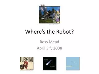
Where’s the Robot?. Ross Mead April 3 rd , 2008. Where’s the Robot?. Given an initial estimate P (0) of the robot’s location in the configuration space , maintain an ongoing estimate of the robot pose P ( t ) at time t with respect to the map. Configuration Space (C-space).

E N D
Where’s the Robot? Ross Mead April 3rd, 2008
Where’s the Robot? • Given an initial estimate P(0) of the robot’s location in the configuration space, maintain an ongoing estimate of the robot pose P(t) at time t with respect to the map.
Configuration Space (C-space) • A set of “reachable” areas constructed from knowledge of both the robot and the world. • How to create it… • abstract the robot as a point object • enlarge the obstacles to account for the robot’s footprint and degrees-of-freedom
Configuration Space (C-space) • Footprint • the amount of space a robot occupies • Degrees-of-Freedom (DoF) • number of variables necessary to fully describe a robot’s “pose” in space • How many DoF does the Create have?
Free Space Obstacles Robot (treat as point object) (x, y, ) Configuration Space (C-space)
“We don’t need no stinkin’ sensors!” • Send a movement command to the robot. • Assume command was successful… • set pose to expected pose following the command • But… robot movement is not perfect… • imperfect hardware (yes… blame hardware… ) • wheel slippage • discrepancies in wheel circumferences • skid steering
different wheeldiameters ideal case carpet bump Reasons for Motion Errors and many more …
What Do We Know About the World? Proprioception Exteroception sensing things about the environment Common exteroceptive sensors are: electromagnetic spectrum sound touch smell/odor temperature range attitude (Inclination) • sensing things about one's own internal status • Common proprioceptive sensors are: • thermal • hall effect • optical • contact
Locomotion • Power of motion from place to place. • Differential drive (Pioneer 2-DX, iRobot Create) • Car drive (Ackerman steering) • Synchronous drive (B21) • Mecanum wheels, XR4000
ICC Instantaneous Center of Curvature (ICC) For rolling motion to occur, each wheel has to move along its y-axis.
Differential Drive • Differences in the velocities of wheels determines the turning angle of the robot. • Forward Kinematics • Given the wheels’ velocities (or positions), what is the robot’s velocity/position ?
Motion Model • Kinematics • The effect of a robot’s geometry on its motion. • If the motors move this much, where will the robot be? • Two types of common motion models: • Odometry-based • Velocity-based (“ded reckoning”) • Odometry-based models are used when systems are equipped with wheel encoders. • Velocity-based models have to be applied when no wheel encoders are given… • calculate new pose based on velocities and time elapsed • in the case of the Creates, we focus on this model
Ded Reckoning “Do you mean, ‘dead reckoning’”?
Ded Reckoning • That’s not a typo… • “ded reckoning” = deduced reckoning • reckon to determine by reference to a fixed basis • Keep track of the current position by noting how far the robot has traveled on a specific heading… • used for maritime navigation • uses proprioceptive sensors • in the case of the Creates, we utilize velocity control
Ded Reckoning • Specify system measurements… • consider possible coordinate systems • Determine the point (radius) about which the robot is turning… • to minimize wheel slippage, this point (the ICC) must lie at the intersection of the wheels’ axles • Determine the angular velocityω at which the robot is turning to obtain the robot velocity v… • each wheel must be traveling at the same ω about the ICC • Integrate to find position P(t)… • the ICC changes over time t
Ded Reckoning y Of these five, what’s known and what’s not? w ICC vl q Thus, R x (x, y) vr (vrand vl in mm/sec)
Ded Reckoning ICC R or P(t+t) P(t)
Ded Reckoning ICC R or P(t+t) P(t) This is kinematics… Sucks,… don’t it… ?
(Adding It All Up) • Update the wheel velocities and, thus, robot velocity information at each sensor update… • How large can/should a single segment be?
Example Move Function // move x centimeters (x > 0), // vel in mm/sec (-500 to 500) void move(float x, intvel) // move is approximate { int dist = (int)(x * 10.0); // change cm to mm create_distance(); // update Create internal distance gc_distance = 0; // and initialize IC’s distance global msleep(50L); // pause before next signal to Create if (dist != 0) { create_drive_straight(vel); if (vel > 0) while (gc_distance < dist) create_distance(); else while (gc_distance > -dist) create_distance(); msleep(50L); // pause between distance checks } create_stop(); // stop } // move(float, int)
Example Turn Function // deg > 0 turn left (CCW), // deg < 0 turn right (CW), // vel in mm/sec (0 to 500) void turn(int deg, intvel) // turn is approximate { create_angle(); msleep(50L); // initialize angle gc_total_angle = 0; // and update IC’s angle global if (deg > 0) { create_spin_CCW(vel); while (gc_total_angle < deg) { create_angle(); msleep(50L); } } else { create_spin_CW(vel); while (gc_total_angle > deg) { create_angle(); msleep(50L); } } create_stop(); // stop } // turn(int, int)
Putting It All Together • How can we modify move(..) and turn(..) to implement ded reckoning to maintain the robot’s pose at all times? • I leave this to you as an exercise…
Types of Mobile Robot Bases Holonomic Non-holonomic A robot is non-holonomic if it can not move to change its pose instantaneously in all available directions. • A robot is holonomic if it can move to change its pose instantaneously in all available directions.
Types of Mobile Robot Bases • Ackerman Drive • typical car steering • non-holonomic
Types of Mobile Robot Bases • Omni Drive • wheel capable of rolling in any direction • robot can change direction without rotating base • Synchro Drive
Dead Reckoning • Ded reckoning makes hefty assumptions… • perfect traction with ground (no slippage) • identical wheel circumferences • ignores surface area of wheels (no skid steering) • sensor error and uncertainty…
What’s the Problem? • Sensors are the fundamental input for the process of perception… • therefore, the degree to which sensors can discriminate the world state is critical • Sensor Aliasing • many-to-one mapping between environmental states to the robot’s perceptual inputs • amount of information is generally insufficient to identify the robot’s position from a single reading
What’s the Problem? • Sensor Noise • adds a limitation on the consistency of sensor readings • often the source of noise is that some environmental features are not captured by the robot’s representation • Dynamic Environments • Unanticipated Events • Obstacle Avoidance
Localization Where am I? ? robot tracking robot kidnapping local problem global problem
Localization Only local data! (even perfect data) robot tracking robot kidnapping local problem global problem
Localization Direct map-matching can be overwhelming robot tracking robot kidnapping local problem global problem
Monte Carlo Localization (MCL) Key idea: keep track of a probability distribution for where the robot might be in the known map Where’s this? Initial (uniform) distribution black - blue - red - cyan
Monte Carlo Localization (MCL) Key idea: keep track of a probability distribution for where the robot might be in the known map blue Initial (uniform) distribution Intermediate stage 1 black - blue - red - cyan
Monte Carlo Localization (MCL) Key idea: keep track of a probability distribution for where the robot might be in the known map blue red Initial (uniform) distribution Intermediate stage 2 black - blue - red - cyan
Monte Carlo Localization (MCL) Key idea: keep track of a probability distribution for where the robot might be in the known map cyan Initial (uniform) distribution Intermediate stages Final distribution black - blue - red - cyan But how?
Deriving MCL Bag o’ tricks p( B | A ) • p( A ) • Bayes’ rule p( A | B ) = p( B ) • Definition of conditional probability p( A B ) = p( A | B ) • p(B) • Definition of marginal probability S p( A ) = p( A B ) all B What are these saying? S p( A ) = p( A | B ) • p(B) all B
! Setting Up the Problem The robot does (or can be modeled to) alternate between • sensing -- getting range observations o1, o2, o3, …, ot-1, ot • acting -- driving around (or ferrying?) a1, a2, a3, …, at-1 “local maps” whence? We want to know P(t) -- the pose of the robot at time t • but we’ll settle for p(P(t)) -- a probability distribution for P(t) What kind of thing is p(P(t)) ? We do know m-- the map of the environment (or will know) p( o | r, m ) -- the sensor model p( rnew | rold, a, m ) -- the motion model = the accuracy of performing action a
Sensor Model map m and location r p( o | r, m ) sensor model p( rnew | rold, a, m )action model p( | r, m ) = .95 p( | r, m ) = .05 potential observationso “probabilistic kinematics” -- encoder uncertainty • red lines indicate commanded action • the cloud indicates the likelihood of various final states
Probabilistic Kinematics We may know where our robot is supposed to be, but in reality it might be somewhere else… Key question: supposed final pose y lots of possibilities for the actual final pose x VL (t) VR(t) starting position What should we do?
Robot Models: How-To p( o | r, m ) sensor model p( rnew | rold, a, m )action model (0) Model the physics of the sensor/actuators (with error estimates) theoretical modeling (1) Measure lots of sensing/action results and create a model from them empirical modeling • take N measurements, find mean (m) and st. dev. (s), and then use a Gaussian model • or, some other easily-manipulated (probability?)model... 0if |x-m| > s 0 if |x-m| > s p( x )= p( x )= 1otherwise 1- |x-m|/sotherwise
Running around in squares MODEL the error in order to reason about it! 3 • Create a program that will run your robot in a square (~2m to a side), pausing after each side before turning and proceeding. • For 10 runs, collect both the odometric estimates of where the robot thinks it is and where the robot actually is after each side. 2 • You should end up with two sets of 30 angle measurements and 40 length measurements: one set from odometry and one from “ground-truth.” 4 • Find the mean and the standard deviation of the differences between odometry and ground truth for the angles and for the lengths – this is the robot’s motion uncertainty model. 1 start and “end” This provides a probabilistic kinematic model.
Monte Carlo Localization (MCL) Start by assuming p( r0 )is the uniform distribution. take K samples of r0 and weight each with a “probability” of 1/K dimensionality?! “Particle Filter” representation of a probability distribution
Monte Carlo Localization (MCL) Start by assuming p( r0 )is the uniform distribution. take K samples of r0 and weight each with a “probability” of 1/K Get the current sensor observation, o1 For each sample point r0multiply the importance factor by p(o1 | r0, m) “probability”
Monte Carlo Localization (MCL) Start by assuming p( r0 )is the uniform distribution. take K samples of r0 and weight each with a “probability” of 1/K Get the current sensor observation, o1 For each sample point r0multiply the importance factor by p(o1 | r0, m) Normalize (make sure the importance factors add to 1) You now have an approximation of p(r1 | o1, …, m) and the distribution is no longer uniform How did this change?
Monte Carlo Localization (MCL) Start by assuming p( r0 )is the uniform distribution. take K samples of r0 and weight each with a “probability” of 1/K Get the current sensor observation, o1 For each sample point r0multiply the importance factor by p(o1 | r0, m) Normalize (make sure the importance factors add to 1) You now have an approximation of p(r1 | o1, …, m) and the distribution is no longer uniform How did this change? Create new samples by dividing up large clumps each point spawns new ones in proportion to its importance factor
Monte Carlo Localization (MCL) Start by assuming p( r0 )is the uniform distribution. take K samples of r0 and weight each with a “probability” of 1/K Get the current sensor observation, o1 For each sample point r0multiply the importance factor by p(o1 | r0, m) Normalize (make sure the importance factors add to 1) You now have an approximation of p(r1 | o1, …, m) and the distribution is no longer uniform How did this change? Create new samples by dividing up large clumps each point spawns new ones in proportion to its importance factor The robot moves, a1 For each sample r1, move it according to the model p(r2 | a1, r1, m) Where do the purple ones go?
Monte Carlo Localization (MCL) Start by assuming p( r0 )is the uniform distribution. take K samples of r0 and weight each with a “probability” of 1/K Get the current sensor observation, o1 For each sample point r0multiply the importance factor by p(o1 | r0, m) Normalize (make sure the importance factors add to 1) You now have an approximation of p(r1 | o1, …, m) and the distribution is no longer uniform How did this change? Create new samples by dividing up large clumps each point spawns new ones in proportion to its importance factor The robot moves, a1 For each sample r1, move it according to the model p(r2 | a1, r1, m) Increase all the indices by 1 and keep going! Where do the purple ones go?