Faults and fault-tolerance
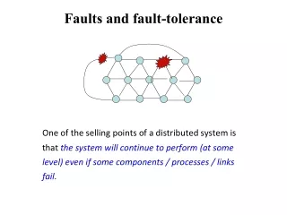
One of the selling points of a distributed system is that the system will continue to perform (at some level) even if some components / processes / links fail. Faults and fault-tolerance. Cause and effect. Study examples of what causes what .

Faults and fault-tolerance
E N D
Presentation Transcript
One of the selling points of a distributed system is that the system will continue to perform (at some level) even if some components / processes / links fail. Faults and fault-tolerance
Cause and effect • Study examples of what causes what. • We view the effect of failures at our level of abstraction, and then try to mask it, or recover from it. • Reliability and availability • MTBF (Mean Time Between Failures) and MTTR (Mean Time To Repair) are two commonly used metrics in the engineering world
A classification of failures • Crash failure • Omission failure • Transient failure • Software failure • Security failure • Byzantine failure • Temporal failure • Environmental perturbations
Crash failures Crash failure = the process halts. It is irreversible. Crash failure is a form of “nice” failure. In a synchronous system, it can be detected using timeout, but in a asynchronous system, crash detection becomes tricky. Some failures may be complex and nasty. Fail-stop failure is a simple abstraction that mimics crash failure when process behavior becomes arbitrary. Implementations of fail-stop behavior help detect which processor has failed. If a system cannot tolerate fail-stop failure, then it cannot tolerate crash.
Omission failures Message lost in transit. May happen due to various causes, like • Transmitter malfunction • Buffer overflow • Collisions at the MAC layer • Receiver out of range
Transient failure (Hardware)Arbitrary perturbation of the global state. May be induced by power surge, weak batteries, lightning, radio-frequency interferences, cosmic rays etc. (Software) Heisenbugs are a class of temporary internal faults and are intermittent. They are essentially permanent faults whose conditions of activation occur rarely or are not easily reproducible, so they are harder to detect during the testing phase. Over 99% of bugs in IBM DB2 production code are non-deterministic and transient (Jim Gray) Not Heisenberg
Software failures Coding error or human error On September 23, 1999, NASA lost the $125 million Mars orbiter spacecraft because one engineering team used metric units while another used English units leading to a navigation fiasco, causing it to burn in the atmosphere. Design flaws or inaccurate modeling Mars pathfinder mission landed flawlessly on the Martial surface on July 4, 1997. However, later its communication failed due to a design flaw in the real-time embedded software kernel VxWorks. The problem was later diagnosed to be caused due to priority inversion, when a medium priority task could preempt a high priority one.
Software failures (continued) Memory leak Operating systems may crash when processes fail to entirely free up the physical memory that has been allocated to them. This effectively reduces the size of the available physical memory over time. When this becomes smaller than the minimum memory needed to support an application, it crashes. Incomplete specification (example Y2K) Year = 09 (1909 or 2009 or 2109)? Many failures (like crash, omission etc) can be caused by software bugs too.
Temporal failures Inability to meet deadlines – correct results are generated, but too late to be useful. Very important in real-time systems. May be caused by poor algorithms, poor design strategy or loss of synchronization among the processor clocks.
Environmental perturbations Consider open systems or dynamic systems. Correctness is related to the environment. If the environment changes, then a correct system becomes incorrect. Example of environmental parameters: time of day, network topology, user demand etc. Essentially, distributed systems are expected to adapt to the environment A system of Traffic lights Time of day
Security problems Security loopholes can lead to failure. Code or data may be corrupted by security attacks. In wireless networks, rogue nodes with powerful radios can sometimes impersonate for good nodes and induce faulty actions.
Byzantine failure Anything goes! Includes every conceivable form of erroneous behavior. It is the weakest type of failure. Numerous possible causes. Includes malicious behaviors (like a process executing a different program instead of the specified one) too. Most difficult kind of failure to deal with.
Specification of faulty behavior (Most faulty behaviors can be modeled as a fault action F superimposed on the normal action S. This is for specification purposes only) program example1; define x : boolean (initially x = true); {a, b are messages); do {S}: x send a {specified action} [] {F}:true send b{faulty action} od a a a a b a a a b b a a a a a a a …
F-intolerant vs F-tolerant systems Four types of tolerance: - Masking - Non-masking - Fail-safe - Graceful degradation tolerances Fault-tolerance A system that tolerates failure of type F faults
P is the invariant of the original fault-free system Q represents the worst possible behavior of the system when failures occur. It is called the fault span. Q is closed under S or F. Fault-tolerance Q P
Masking tolerance: P = Q (neither safety nor liveness is violated) Non-masking tolerance: P Q (safety property may be temporarily violated, but not liveness). Eventually safety property is restored. Fault-tolerance Q P
Classifying fault-tolerance Masking tolerance. Application runs as it is. The failure does not have a visible impact. All properties (both liveness & safety) continue to hold. Non-masking tolerance. Safety property is temporarily affected, but not liveness. Example1. Clocks lose synchronization, but recover soon thereafter. Example 2. Multiple processes temporarily enter their critical sections, but thereafter, the normal behavior is restored. Example3. A transaction crashes, but eventually recovers
Backward vs. forward error recovery These are two forms of non-masking tolerance: Backward error recovery When safety property is violated, the computation rolls back and resumes from a previous correct state. time rollback Forward error recovery Computation does not care about getting the history right, but moves on, as long as eventually the safety property is restored. True for self-stabilizing systems.
Classifying fault-tolerance Fail-safe tolerance Given safety predicate is preserved, but liveness may be affected Example. Due to failure, no process can enter its critical section for an indefinite period. In a traffic crossing, failure changes the traffic in both directions to red. Graceful degradation Application continues, but in a “degraded” mode. Much depends on what kind of degradation is acceptable. Example. Consider message-based mutual exclusion. Processes will enter their critical sections, but not in timestamp order.
Failure detection The design of fault-tolerant systems will be easier if failures can be detected. Depends on the 1. System model, and 2. The type of failures. Asynchronous models are more tricky. We first focus on synchronous systems only
Detection of crash failures Failure can be detected using heartbeat messages (periodic “I am alive” broadcast) and timeout - if processors speed has a known lower bound - channel delays have a known upper bound. True for synchronous models only. We will address failure detectors for asynchronous systems later.
Detection of omission failures For FIFO channels: Use sequence numbers with messages. (1, 2, 3, 5, 6 … ) ⇒ message 5 was received but not message 4 ⇒ message must be is missing Non-FIFO bounded delay channels delay - use timeout (Message 4 should have arrived by now, but it did not) What about non-FIFO channels for which the upper bound of the delay is not known? -- Use sequence numbers and acknowledgments. But acknowledgments may also be lost. We will soon look at a real protocol dealing with omission failure ….
Detection of transient failures The detection of an abrupt change of state from S to S’ requires the periodic computation of local or global snapshots of the distributed system. The failure is locally detectable when a snapshot of the distance-1 neighbors reveals the violation of some invariant. Example: Consider graph coloring
Detection of Byzantine failures Feasible in some limited cases, using witnesses and reaching consensus In case (b), B is malicious, but in (c) B is ignorant. A system with 3f+1 processes is considered adequate for (sometimes) detecting (and definitely masking) up to f byzantine faults.
It is possible to tolerate f crash failures using (f+1) servers. So for tolerating a single crash failure, Double Modular Redundancy (DMR) is adequate Tolerating crash failures Faulty replicas User querying the replica servers
Triple modular redundancy (TMR) for masking any single failure. Triple Modular Redundancy x User takes a vote x’ x N-modular redundancy masks up to m failures, when N = 2m +1
A central issue in networking Tolerating omission failures router A Routers may drop messages, but reliable end-to-end transmission is an important requirement. If the sender does not receive an ack within a time period, it retransmits (it may so happen that the was not lost, so a duplicate is generated). This implies, the communication must tolerate Loss, Duplication, and Re-ordering of messages B router
{program for process S} define ok : boolean; next : integer; initially next = 0, ok = true, both channels are empty; do ok send (m[next], next); ok:= false [] (ack, next) is received ok:= true; next := next + 1 [] timeout (R,S) send (m[next], next) od {program for process R} define r : integer; initially r = 0; do (m[ ], s) is received s = r accept the message; send (ack, r); r:= r+1 [] (m[ ], s) is received s ≠ r send (ack, r-1) od Stenning’s protocol Sender S next ok m[0], 0 ack r Receiver R
Both messages and acks may be lost Q. Why is the last ack reinforced by R when s≠r? A. Needed to guarantee progress. Progress is guaranteed, but the protocol is inefficient due to low throughput. Observations on Stenning’s protocol Sender S m[0], 0 ack Receiver R
Observations on Stenning’s protocol Sender S (s =1) If the last ack is not reinforced by the receiver when s≠r, then the following scenario is possible But it is lost m[1], 1 -- The ack of m[1] is lost. -- After timeout, S sends m[1] again. -- But R was expecting m[2], so does not send ack. And S keeps sending m[1] repeatedly. This affects progress. ack Receiver R (r=2)
Sliding window protocol • The sender continues the send action • without receiving the acknowledgements of at most • w messages (w > 0), w is called the window size.
{program for process S} define next, last, w : integer; initially next = 0, last = -1, w > 0 do last+1 ≤ next ≤ last + w send (m[next], next); next := next + 1 [] (ack, j) is received if j > last last := j [] j ≤ last skip fi [] timeout (R,S) next := last+1 {retransmission begins} od {program for process R} define j : integer; initially j = 0; do (m[next], next) is received if j = next accept message; send (ack, j); j:= j+1 [] j ≠ next send (ack, j-1) fi; od Sliding window protocol
Example Window size =5 (last= -1) 4, 3, 2, 1, 0 (2 is lost) 4, 1, 3, 0 S R (j=0) (next=5) (m[0, m[1] accepted, but m[3]-m[4] are not) 4, 1, 3 (last= -1) 4, 3, 2, 1, 0 (2 is lost) S R (j=2) (next=5) 0, 0, 1, 1 For j ≠ next For message 0 (last= 1) 6, 5, 4, 3, 2 S R (j=2) (next=5) timeout
Observations Lemma. Every message is accepted exactly once. (Note the difference between reception and acceptance) Lemma. Message m[k] is always accepted before m[k+1]. (Argue that these are true. Consider various scenarios of omission failure) Uses unbounded sequence number. This is bad. Can we avoid it?
Theorem If the communication channels are non-FIFO, and the message propagation delays are arbitrarily large, then using bounded sequence numbers, it is impossible to design a window protocol that can withstand the (1) loss, (2) duplication, and (3) reordering of messages.
Why unbounded sequence no? (m’’,k) (m’, k) (m[k],k) New message using the same seq number k Retransmitted version of m We want to accept m” but reject m’. How is that possible?
Alternating Bit Protocol m[1],1 m[0],0 m[0],0 R S ack, 0 ABP is a link layer protocol. Works on FIFO channels only. Guarantees reliable message delivery with a 1-bit sequence number (this is thetraditional version with window size = 1). Study how this works.
Alternating Bit Protocol programABP; {program for process S} define sent, b : 0 or 1; next : integer; initially next = 0, sent = 1, b = 0, and channels are empty; do sent ≠ b send (m[next], b); next := next+1; sent := b [] (ack, j) is received if j = b b := 1- b [] j ≠ b skip fi [] timeout (R,S) send (m[next-1], b) od {program for process R} define j : 0 or 1; {initially j = 0}; do (m[ ], b) is received if j = b accept the message; send (ack, j); j:= 1 - j [] j ≠ b send (ack, 1-j) fi od S m[1],1 a,0 m[0],0 m[0],0 R
How TCP works Three-way handshake. Sequence numbers are unique w.h.p.
TCP sequence numbers Supports end-to-end logical connectionbetween any two computers on the Internet. Basic idea is the same as those of sliding window protocols. But TCP uses bounded sequence numbers (32 or 64 bits)! The primary issue here is to prevent another connection from reusing an existing sequence number, such re-use may open the door for an attack. By correctly guessing (or acquiring) an existing sequence number, the attacker may inject arbitrary messages that will be accepted by the receiver as valid messages from the sender. The use of a random initial sequence numbers by the sender and the receiver prevents it.
TCP sequence numbers There is the potential of old packets with sequence numbers belonging to an acceptable window appearing into the system. These are prevented by automatically killing old packets (using TTL) after a time = 2d, where d is the round trip delay.
How TCP works: Various Issues • Why is the knowledge of roundtrip delay important? • --Timeout can be correctly chosen • What if the timeout period is too small / too large? • -- • What if the window is too small / too large? • -- • Adaptive retransmission: receiver can throttle sender • and control the window size to save its buffer space.