Download
1 / 42
420 likes | 858 Vues
UCL ECON7003 Money and Banking. “008-9. Topic 7. Monetarism. Monetary policy in post-war period. Limited debate. Practical problems. Beginnings of monetarist critique. Return of macroeconomic turbulence: debate revives. Monetarist theory.

E N D
UCL ECON7003 Money and Banking. “008-9.Topic 7.Monetarism. • Monetary policy in post-war period. • Limited debate. Practical problems. Beginnings of monetarist critique. Return of macroeconomic turbulence: debate revives. • Monetarist theory. • Friedman: Quantity Theory of Money restated. Permanent Income Hypothesis. Adaptive Expectations Hypothesis. LR / SR distinction. ‘Natural rate’. • Monetary policy ‘in’ the ISLM framework. • Money market disequilibrium. Discretionary MP and generation of Cycle. ‘Long and variable lags’. • Optimum MS rule. • Problems of CB in controlling MS – review and preview.
Monetary policy in post-war boom: • High war debts → government aims: • Keep down government’s r repayments • Maintain PB. • Curb effects by ceilings on credit / credit rationing. • Low π: • Fixed ER (Bretton Woods) till early 1970s. • Counter-inflationary policy: ‘prices and incomes policy’ > monetary instruments. • Outcome: Bias towards loose monetary policy. • → Steady build-up of underlying inflationary pressure.
Monetarist critique: • ‘Monetarists’’ (Friedman, Chicago school) seen as ‘fringe’ in post-war years. • Criticised view that monetary policy is relatively unimportant / secondary / ‘accommodating’ role only, i.e. the Keynesian view that: • ΔM → Δr → Δi, BUT this effect quite weak: Flattish LM Steep IS / I r-inelastic • LR factors > SR Δr, i.e.. • Friedman: ‘twice damned’. • Called for more debate on monetary policy / ‘money matters’.
Monetary policy “twice damned”: IS aspect – review. • Monetarism: IS flattish: • I highly r-sensitive. • Slope represents marginal efficiency of capital. • i.e. S-side influences on investment demand. • Keynesianism: IS steep. • r is only one among many determinants of I. • Likely to be relatively minor. • Decisions likely to be very LR. • i.e. not dependent on SR factors like fluctuations in r.
Friedman (1968): ‘twice damned’. • “If liquidity preference is absolute or nearly so – as Keyes believed likely in times of heavy unemployment – interest rates cannot be lowered by monetary measures. • “If investment and consumption are little affected by interest rates… lower interest rates, even if they could be achieved, would do little good. • “Monetary policy is twice damned… • “The wide acceptance of these views in the economics profession meant that for some two decades monetary policy was believed by all but a few reactionary souls to have been rendered obsolete by new economic knowledge.”
Practical problems with post-war UK macro policy: • Balance of Payments / conflict of goals. • £ fixed against $ at rate unchanged for 18 years ($2.80 / £). • This constrained MP: • Expansion [GO!] → BOP deficit: M↑, X↓. • → response: deflation [STOP!] , with goal of: • Imports ↓ • π↓ → export competitiveness↑ • When BOP back to surplus, government would reflate [GO!]. • i.e. ‘stop-go’.
High output, low unemployment but high inflation, current account deficit Low inflation, current account surplus but low output, high unemployment Problems of ‘stop-go’: Conflict of policy goals: BOP and the domestic cycle BUT: Say c/a deficit is persistent – long term downward trend –STOP! or GO! ?? Y high BUT: → M↑andπ also high→ X↓ BOP deficit → STOP! π low but Y also low→ GO! → π back up again National output Time
1960s: conflict of goals / domestic and international priorities: • Underlying problem: UK’s exports increasingly uncompetitive. • → Continuous underlying problem of BOP deficit. • → LR pressure for the appropriate deflationary policy / “STOP!”. • ≡ downward pressure on £. • But eventually more pronounced slowdown > fluctuations. • → Intensifying conflict with domestic cycle: need for “GO!”. • 1967: UK forced to devalue £ to alleviate BOP problem. • i.e. Rather than more “STOP!”. • Preview: Another conflict of goals episode: late 1980s-1992.
Post-war ‘consensus’ always uneasy. e.g. Conservative cabinet split in 1957-8. Meanwhile, ‘monetarism’ of Friedman / Chicago school laying theoretical base: • monetary policy should be taken seriously: • not for any good it might do • but for harm if misguidedly adopted as tool for DMP.
Late 1960s developing macro instability: Persistent BOT deficit Inflation edging up BOP crisis and devaluation 1967. • Response of Heath government of 1970-4: • ‘Free market’ policies • But these backfired. • In particular, intensified the inflationary pressures.
Inflationary pressures, early 1970s: • Sweeping deregulation– ‘Competition and Credit Control’. → Dramatic increase in credit and MS. • 1972-3: ‘Last fling’ of loose monetary and fiscal policy from a Conservative government (‘Barber boom’). • Breakdown of Bretton Woods → ER no longer a restraint on MS. • Strong pressure for W increases. • π already soaring when overtaken by oil pricerise late 1973.
Heath government reverted to interventionist counter-measures: • ‘Prices and income’ policies. • Seen as unsuccessful. • Conservative government fell 1974. • → Split in Conservative Party and adoption of Thatcher as Party leader in 1975. • Monetarism -- influential advocates: • In press – writers / editors in Financial Times, Times. • In right wing of Tory Party (Powell, Joseph). • Thatcher became figurehead during late 1970s.
Phillips curve. • Unemployment and (wage) inflation, 1861-1913. • From Phillips’s 1958 article. BUT: Labour government of 1974-9 faced: • ‘Stagflation’. • i.e. breakdown of Phillips curve relationship.
65 68 66 61 64 63 60 Breakdown of the stable Phillips Curve π (%) 75 From late 1960s, negative relationship between u and π no longer evident 80 76 74 77 79 81 90 71 73 82 89 78 72 70 91 85 69 84 88 83 87 62 95 86 92 97 00 98 94 67 96 01 93 02 99 u
Labour government reintroduced P&I policies. • Some success against π, but £ continued to fall: • 1976-7: forced to accept monetarist conditions for IMF loan: • Money supply targets. • Market oriented supply-side measures: • tax reform • union reform • abandonment of minimum W • reduction in UB • cuts in public services. • Monetarist policies in UK thus associated with market-oriented / S-side approach / ‘cuts’: • Conservatives more ideologically in tune than Labour. • Won election of May 1979 on ‘monetarist’ platform.
Friedman’s restatement of QTM. • Keynesianism (ISLM version!) made simplifying assumption: • M and B the only two assets affecting money demand. • i.e. Bonds the only alternative to holding M. • Friedman: No -- other assets apart from bonds also need to be taken into account, e.g. • residential and other property • consumer-durables • equities, etc. • These are also held as alternatives to money.
Friedman: • r is relatively insignificant in determining MD. • Affects money-versus-bonds decision. • BUT: Various other influences also (contra Keynesian limiting assumption): • Some positive, some negative. • May net to zero. • MD is thus overall interest-rate-inelastic.
Cambridge: • MD = kPY • k is factor of proportionality / ‘Marshallian’ or ‘Cambridge’ k. • Reformulates QTM as theory of money demand. • Keynes: • MD = k(r).PY • Not compatible with QTM. • k not constant – cyclical fluctuations, etc. • Friedman: • MD = k(rB, r1 . . . rn).PY • rB: return on bonds • r1 . . . rn : rates of return (explicit or implicit) on other assets besides bonds. These net out → k = ki.e. Restatement of QTM.
Friedman: • Income may fluctuate (cycle, etc.), so how justify concept of stable MD? • Individuals smooth out expenditure: • ‘Permanent Income’: • Saving / dis-saving over perceived / expected average lifetime earning. • i.e. MD responds to wealth, as flow > stock variable. • Money demand has a stable relation to wealth, thus defined.
Neutrality of money – LR / SR distinction: • ‘Old’ QTM: • ΔM → ΔP only, with ΔY = 0. • i.e. ΔP / ΔM = 1. • Friedman: M is neutral in LR, as in old QTM: • i.e. ΔLRP / ΔM = 1. • BUT: ΔM may have SR effect on Y: • ΔM → ΔP, but alsoΔSRY > 0. • i.e. ΔSRP / ΔM < 1. • This SR effect gradually unwinds till we have • ΔLRP / ΔM = 1.
Friedman’s Adaptive Expectations Hypothesis / ‘fooling’ model / effect of SR changes in MS: • Wage-earners’ expectations of movements in P take time to adapt. • P↑ and wage-earners underestimate change. • → they supply more labour than if they had realised how much their real wage has been eroded by inflation. • Model works symmetrically in reverse / overestimation.
Friedman’s monetarism: adaptive expectations, and the LR-SR distinction, contd • Workers supply more labour → Y↑ because they think their real wage has increased more than it actually has. P’ AD1 MS ↑ → AD ↑ Y’ P LRAS SRAS (Pe = P0) P0 AD0 Y* Y
Friedman’s monetarism: adaptive expectations, and the LR-SR distinction, contd SRAS (Pe = P1) P1 (2) P LRAS (Pe = P) SRAS (Pe = P0) Workers realise they have overestimated their real wage and adjust it over successive time periods, so they reduce LS, i.e. AS shifts left. AD1 P0 (1) Eventually Y returns to Y* AD0 Y’ Y* Y
P has risen, and Y falls back to its original level – the ‘Natural Rate’. Friedman’s monetarism: adaptive expectations, and the LR-SR distinction, contd LRAS (Pe = P) SRAS (Pe = P1) P Y returns to YNR -- net result is ΔP only SRAS (Pe = P0) P1 P0 AD1 AD0 Net result is just inflation and instability. YNR Y
≡ the ‘short run’ P, Pe P Pe t
‘Natural rate’ • ‘Old’ classical: • Unique point of equilibrium / self-regulating level. • This is YFE. • Friedman: This is unrealistic. • → redefined LR sustainable level as ‘natural rate’: • (1) Will always be some u. • At equilibrium / self-sustaining level: ‘natural rate’ – NRU. • (2) NRU is not constant. • Changes with changing labour market conditions.
Money market equilibrium with monetarist assumptions: • MS exogenous. • MD a stable function of income. • Unique point of equilibrium: • MD/P(ye) = MS/P • MS curve super-imposedon MD curve.
Disequilibrium in money market on monetarist assumptions. • With MD at MD0/P (MD1/P), r rise (fall) without limit. • Keynesianism: r determined in money market. • Monetarism: r undetermined in money market.
Effects of discretionary monetary policy -- monetarist view. • Discretionary monetary policy → Downward (upward) pressure on r. • → MS above (below) unique level appropriate to ye • → y deviates above (below) ye. • All points where y ≠ ye are off money market equilibrium. • LM is stationary at unique position appropriate to ye.
NOTE ALSO: • Keynes himself (unlike ISLM version?): • Un-modellable D-side factors: • Mood (investor optimism, pessimism). • Expectations. • Volatility. • “Human decisions affecting the future … cannot depend on strict mathematical expectation… the outcome of a weighted average of quantitative benefits multiplied by quantitative probabilities. • [We act] “choosing between the alternatives as best we are able, calculating where we can, but often falling back for our motive on whim or sentiment or chance”.
GDP Volatility of Investment greater than Volatility of GDP Sloman p. 487, Box 17.6 Investment GDP fig
Discretionary MP and generation of cycle: monetarist view. Monetary expansion → r↓ → economy moves down IS. Monetary contraction is then implemented as a counter-measure. BUT overshoots ye.
‘Long and variable lags’ in effects of discretionary monetary policy. • → Impossible to stabilise AD through this means. • Expansions and contractions in themselves net to zero. • But outcome nevertheless adverse -- economy harmed by instability. • Discretionary monetary policy is principal cause of business cycle.
Path (b) – aim of intervention, i.e. Keynesian DMP Path (c) – undesired outcome, i.e. Monetarist critique. Fluctuations and lags Path (a) – without intervention Y The intervention has increased the amplitude of the fluctuations! O Time
Monetarist alternative to discretionary monetary policy: • Should be conducted according to a rule. • Any rule is better than discretion. • Friedman’s preference: • Constant money growth rule: • Growth rate set according to LR growth rate of economy.
Monetarism’s optimal MS rule: • Set growth rate of M at same rate as growth of Y. • → MR equilibrium: • MV = PY • MR: y = ye + classical assumption of V = V • → P = V/Y.M = const. x M, say κM, i.e. QTM. • π ≡ (P – P-1) / P-1 • = (κM – κM -1) / κM -1 • = (M – M -1) / M -1 • i.e. MR equilibrium: • π = γ, where γ is growth rate of M.
LR economic growth → ΔMS is necessary • BUT MS should be set in way that minimises inflationary expectations. • Governments cannot be trusted with discretion to do this: • they have other motives. • → Monetary policy should be set by rules that are • clearly-identifiable • publicly-announced • credibly enforceable • e.g. in step with the trend rate of growth. • Should be administered by a monetary authority independent of government.
Money market: • ye to ye′ determined on S-side. • → MD increases from MD(ye) to MD(ye′). • CB follows its MS growth rule • → MS = MD, i.e. superimposed. • → no upward or downward pressure on r.
r not determined in M Market, but by 3-way interaction between: D-side influences (represented by IS curve); S-side constraints (represented by Phillips Curve); CB preferences w.r.t. trade-off between u and π(see WS6).
Non-inflationary increase in MS by CB following MS rule in low-π conditions – preview.
i.e. no upward or downward pressure on r from money market. • → LM curve ceases to act as constraint. • r determined by 3-way interaction from elsewhere.
BUT: Problems of CB in controlling MS – review and preview. • CB is not the only player in MS process: • Decisions of commercial banks over deposit creation / excess reserves, etc. • Decisions of NBP affect cash-deposit ratio. • Decisions of borrowers from banks affect interest rates. → Next lecture: The historical experience of targeting monetary aggregates.