Download

1 / 65
650 likes | 693 Vues
Learn about the Bernoulli and Binomial distributions, how to estimate population parameters, and their mean and variance. Explore related concepts like the Poisson distribution, unbiased estimates, and estimation uncertainty.

E N D
Commonly Used Distributions Berlin Chen Department of Computer Science & Information Engineering National Taiwan Normal University Reference: 1. W. Navidi. Statistics for Engineering and Scientists. Chapter 4 & Teaching Material
Population Sample Inference Statistics Parameters How to Estimate Population (Distribution) Parameters ? - Unbiased Estimate ? - Estimation Uncertainty ?
The Bernoulli Distribution • We use the Bernoulli distribution when we have an experiment which can result in one of two outcomes • One outcome is labeled “success,” and the other outcome is labeled “failure” • The probability of a success is denoted by p. The probability of a failure is then 1 – p • Such a trial is called a Bernoulli trial with success probability p
Examples • The simplest Bernoulli trial is the toss of a coin. The two outcomes are heads and tails. If we define heads to be the success outcome, then p is the probability that the coin comes up heads. For a fair coin, p = ½ • Another Bernoulli trial is a selection of a component from a population of components, some of which are defective. If we define “success” to be a defective component, then p is the proportion of defective components in the population
X ~ Bernoulli(p) • For any Bernoulli trial, we define a random variable X as follows: • If the experiment results in a success, then X = 1. Otherwise, X = 0. It follows that X is a discrete random variable, with probability mass function p(x) defined by p(0) = P(X = 0) = 1 – p p(1) = P(X = 1) = p p(x) = 0 for any value of x other than 0 or 1
Mean and Variance of Bernoulli • If X ~ Bernoulli(p), then • X = 0(1- p) + 1(p) = p
The Binomial Distribution • If a total of n Bernoulli trials are conducted, and • The trials are independent • Each trial has the same success probability p • X is the number of successes in the n trials Then X has the binomial distribution with parameters n and p, denoted X ~ Bin(n,p) Probability Histogram Bin(10, 0.4) Bin(20, 0.1)
Another Use of the Binomial • Assume that a finite population contains items of two types, successes and failures, and that a simple random sample is drawn from the population. Then if the sample size is no more than 5% of the population, the binomial distribution may be used to model the number of successes • Sample items can be therefore assumed to be independent of each other • Each sample item is a Bernoulli trial
pmf, Mean and Variance of Binomial • If X ~ Bin(n, p), the probability mass function of X is • Mean: X = np • Variance:
More on the Binomial • Assume n independent Bernoulli trials are conducted • Each trial has probability of success p • Let Y1, …, Ynbe defined as follows: Yi= 1 if the ith trial results in success,and Yi = 0 otherwise (Each of the Yi has the Bernoulli(p) distribution) • Now, let X represent the number of successes among the n trials. So, X = Y1 + …+ Yn This shows that a binomial random variable can be expressed as a sum of Bernoulli random variables
Estimate of p • If X ~ Bin(n, p), then the sample proportion is used to estimate the success probability p • Note: • Bias is the difference • is unbiased • The uncertainty in is • In practice, when computing , we substitute for p, since p is unknown
The Poisson Distribution • One way to think of the Poisson distribution is as an approximation to the binomial distribution when n is large and p is small • It is the case when n is large and p is small the mass function depends almost entirely on the mean np, very little on the specific values of n and p • We can therefore approximate the binomial mass function with a quantity λ = np;this λ is the parameter in the Poisson distribution
pmf, Mean and Variance of Poisson • If X ~ Poisson(λ), the probability mass function of X is • Mean: X = λ • Variance: • Note: X must be a discrete random variable and λ must be a positive constant Probability Histogram Poisson(10) Poisson(1)
Relationship between Binomial and Poisson • The Poisson PMF with parameter is a good approximation for a binomial PMF with parameters and , provided that , is very large and is very small
Poisson Distribution to Estimate Rate • Let λdenote the mean number of events that occur in one unit of time or space. Let X denote the number of events that are observed to occur in t units of time or space • If X ~ Poisson(λt), we estimate λwith • Note: • is unbiased ( ) • The uncertainty in is • In practice, we substitute for λ, since λ is unknown
Some Other Discrete Distributions • Consider a finite population containing two types of items, which may be called successes and failures • A simple random sample is drawn from the population • Each item sampled constitutes a Bernoulli trial • As each item is selected, the probability of successes in the remaining population decreases or increases, depending on whether the sampled item was a success or a failure • For this reason the trials are not independent, so the number of successes in the sample does not follow a binomial distribution • The distribution that properly describes the number of successes is the hypergeometric distribution
pmf of Hypergeometric • Assume a finite population contains N items, of which R are classified as successes and N – R are classified as failures • Assume that n items are sampled from this population, and let X represent the number of successes in the sample • Then X has a hypergeometric distribution with parameters N, R, and n, which can be denoted X ~ H(N,R,n). The probability mass function of X is
Mean and Variance of Hypergeometric • If X ~ H(N, R, n), then • Mean of X: • Variance of X:
Geometric Distribution • Assume that a sequence of independent Bernoulli trials is conducted, each with the same probability of success, p • Let X represent the number of trials up to and including the first success • Then X is a discrete random variable, which is said to have the geometric distribution with parameter p. • We write X ~ Geom(p).
pmf, Mean and Variance of Geometric • If X ~ Geom(p), then • The pmf of X is • The mean of X is • The variance of X is
Negative Binomial Distribution • The negative binomial distribution is an extension of the geometric distribution. Let r be a positive integer. Assume that independent Bernoulli trials, each with success probability p, are conducted, and let X denote the number of trials up to and including the rth success • Then X has thenegative binomial distributionwith parameters r and p. We write X ~ NB(r,p) • Note: If X ~ NB(r,p), then X = Y1 + …+ Yrwhere Y1,…,Yrare independent random variables, each with Geom(p) distribution 0,…, 1, 0,…, 1, 0, …1, ……,0,…..,1 x trials in total yr y1 y2
pmf, Mean and Variance of Negative Binomial • If X ~ NB(r,p), then • The pmf of X is • The mean of X is • The variance of X is
Multinomial Distribution • A Bernoulli trial is a process that results in one of two possible outcomes. A generalization of the Bernoulli trial is the multinomial trial, which is a process that can result in any of k outcomes, where k≥ 2. We denote the probabilities of the k outcomes by p1,…,pk (p1+…+pk=1) • Now assume that n independent multinomial trials are conducted each with k possible outcomes and with the same probabilities p1,…,pk. Number the outcomes 1, 2, …, k. For each outcome i, let Xi denote the number of trials that result in that outcome. Then X1,…,Xk are discrete random variables. The collection X1,…,Xk is said to have the multinomial distribution with parameters n, p1,…,pk. We write X1,…,Xk ~ MN(n, p1,…,pk)
pmf of Multinomial • If X1,…,Xk ~ MN(n, p1,…,pk), then the pmf of X1,…,Xk is • Note that if X1,…,Xk ~ MN(n, p1,…,pk), then for each i, Xi ~ Bin(n, pi) Can be viewed as a joint probability mass function of X1,…,Xk
The Normal Distribution • The normal distribution (also called the Gaussian distribution) is by far the most commonly used distribution in statistics. This distribution provides a good model for many, although not all, continuous populations • The normal distribution is continuous rather than discrete. The mean of a normal population may have any value, and the variance may have any positive value
pmf, Mean and Variance of Normal • The probability density function of a normal population with mean and variance 2 is given by • If X ~ N(, 2), then the mean and variance of X are given by
68-95-99.7% Rule • The above figure represents a plot of the normal probability density function with mean and standard deviation . Note that the curve is symmetric about , so that is the median as well as the mean. It is also the case for the normal population • About 68% of the population is in the interval • About 95% of the population is in the interval 2 • About 99.7% of the population is in the interval 3
Standard Units • The proportion of a normal population that is within a given number of standard deviations of the mean is the same for any normal population • For this reason, when dealing with normal populations, we often convert from the units in which the population items were originally measured to standard units • Standard units tell how many standard deviations an observation is from the population mean
Standard Normal Distribution • In general, we convert to standard units by subtracting the mean and dividing by the standard deviation. Thus, if x is an item sampled from a normal population with mean and variance 2, the standard unit equivalent of x is the number z, where z = (x - )/ • The number z is sometimes called the “z-score” of x. The z-score is an item sampled from a normal population with mean 0 and standard deviation of 1. This normal distribution is called the standard normal distribution
Examples • Q: Aluminum sheets used to make beverage cans have thicknesses that are normally distributed with mean 10 and standard deviation 1.3. A particular sheet is 10.8 thousandths of an inch thick. Find the z-score: Ans.: z = (10.8 – 10)/1.3 = 0.62 • Q: Use the same information as in 1. The thickness of a certain sheet has a z-score of -1.7. Find the thickness of the sheet in the original units of thousandths of inches: Ans.: -1.7 = (x – 10)/1.3 x = -1.7(1.3) + 10 = 7.8
Finding Areas Under the Normal Curve • The proportion of a normal population that lies within a given interval is equal to the area under the normal probability density above that interval. This would suggest integrating the normal pdf; this integral have no closed form solution • So, the areas under the curve are approximated numerically and are available in Table A.2 (Z-table). This table provides area under the curve for the standard normal density. We can convert any normal into a standard normal so that we can compute areas under the curve • The table gives the area in the left-hand tail of the curve • Other areas can be calculated by subtraction or by using the fact that the total area under the curve is 1
Examples • Q: Find the area under normal curve to the left of z = 0.47 Ans.: From the z table, the area is 0.6808 • Q: Find the area under the curve to the right of z = 1.38 Ans.: From the z table, the area to the left of 1.38 is 0.9162. Therefore the area to the right is 1 – 0.9162 = 0.0838
More Examples • Q: Find the area under the normal curve between z = 0.71 and z = 1.28. Ans.: The area to the left of z = 1.28 is 0.8997. The area to the left of z = 0.71 is 0.7611. So the area between is 0.8997 – 0.7611 = 0.1386 • Q: What z-score corresponds to the 75th percentile of a normal curve? Ans.: To answer this question, we use the z table in reverse. We need to find the z-score for which 75% of the area of curve is to the left. From the body of the table, the closest area to 75% is 0.7486, corresponding to a z-score of 0.67
Linear Combinations of Independent Normal RVs • The linear combinations of independent normal random variables are still normal random variables • Let are independent, then is normal with • Mean • Variance • We have to distinguish the meaning of from that of
Estimating the Parameters of Normal • If X1,…,Xn are a random sample from a N(,2) distribution, is estimated with the sample mean and 2 is estimated with the sample variance • As with any sample mean, the uncertainty in which we replace with , if is unknown. The mean is an unbiased estimator of . asymptotically unbiased estimator ? unbiased estimator
Sample Variance is an Asymptotically Unbiased Estimator (1/3) • Sample variance is an asymptotically unbiased estimator of the population variance
Sample Variance is an Asymptotically Unbiased Estimator (2/3) The size of the observed sample
Sample Variance is an Asymptotically Unbiased Estimator (3/3) (a kind of uncertainty)
The Lognormal Distribution • For data that contain outliers (on the right of the axis), the normal distribution is generally not appropriate. The lognormal distribution, which is related to the normal distribution, is often a good choice for these data sets • If X ~ N(,2), then the random variable Y = eXhas the lognormal distribution with parameters and 2 • If Y has the lognormal distribution with parameters and 2, then the random variable X = lnY has the N(,2) distribution a lognormal distribution with parameters Probability Density Function
pdf, Mean and Variance of Lognormal • The pdf of a lognormal random variable with parameters and 2is • The mean E(Y) and variance V(Y) are given by • Can be shown by advanced methods
pdf, Mean and Variance of Lognormal • Recall “Derived Distributions”
Test of “Lognormality” • Transform the data by taking the natural logarithm (or any logarithm) of each value • Plot the histogram of the transformed data to determine whether these logs come from a normal population Probability Histogram taking the natural logarithm on the values of the data
The Exponential Distribution • The exponential distribution is a continuous distribution that is sometimes used to model the time that elapses before an event occurs • Such a time is often called a waiting time • The probability density of the exponential distribution involves a parameter, which is a positive constant λ whose value determines the density function’s location and shape • We write X ~ Exp(λ)
pdf, cdf, Mean and Variance of Exponential • The pdf of an exponential r.v. is • The cdf of an exponential r.v. is • The mean of an exponential r.v. is • The variance of an exponential r.v. is Probability Density Function
Lack of Memory Property for Exponential • The exponential distribution has a property known as the lack of memory property: If T ~ Exp(λ), and t and s are positive numbers, then P(T > t + s | T > s) = P(T > t)
Estimating the Parameter of Exponential • If X1,…,Xn are a random sample from Exp(λ), then the parameter λ is estimated with This estimator is biased. This bias is approximately equal to λ/n (specifically, ). The uncertainty in is estimated with • This uncertainty estimate is reasonably good when the sample size n is more than 20
The Gamma Distribution (1/2) • Let’s consider the gamma function • For r > 0, the gamma function is defined by • The gamma function has the following properties: • If r is any integer, then Γ(r) = (r-1)! • For any r, Γ(r+1) = r Γ(r) • Γ(1/2) =
The Gamma Distribution (2/2) • The pdf of the gamma distribution with parameters r > 0 and λ > 0 is • The mean and variance of Gamma distribution are given by • , respectively • If X1,…,Xr are independent random variables, each distributed as Exp(λ), then the sum X1+…+Xr is distributed as a gamma random variable with parameters r and λ, denoted as Γ(r, λ)