Intelligent Backtracking Algorithms in Constraint Processing (CSCE 421/821 Spring 2009)
500 likes | 631 Vues
This course covers intelligent backtracking algorithms that enhance constraint satisfaction problem (CSP) solving techniques. Focus areas include hybrid backtracking algorithms, variable ordering, and consistency checking. Students will engage with essential readings such as Prosser's hybrid algorithms and Dechter’s chapters, as well as hands-on exercises through notes and discussions. Topics will explore backtracking strategies, conflict-directed backjumping, and empirical evaluations of algorithm performance, preparing participants to apply advanced techniques in real-world problem-solving.

Intelligent Backtracking Algorithms in Constraint Processing (CSCE 421/821 Spring 2009)
E N D
Presentation Transcript
Foundations of Constraint Processing CSCE421/821, Spring 2009: www.cse.unl.edu/~choueiry/S09-421-821/ Berthe Y. Choueiry (Shu-we-ri) Avery Hall, Room 360 choueiry@cse.unl.edu Tel: +1(402)472-5444 Intelligent Backtracking Algorithms
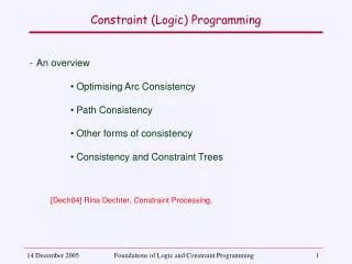
Reading • Required reading Hybrid Algorithms for the Constraint Satisfaction Problem [Prosser, CI 93] • Recommended reading • Chapters 5 and 6 of Dechter’s book • Tsang, Chapter 5 • Notes available upon demand • Notes of Fahiem Bacchus: Chapter 2, Section 2.4 • Handout 4 and 5 of Pandu Nayak (Stanford Univ.)
Outline • Review of terminology of search • Hybrid backtracking algorithms
Backtrack search (BT) • Variable/value ordering • Variable instantiation • (Current) path • Current variable • Past variables • Future variables • Shallow/deep levels /nodes • Search space / search tree • Back-checking • Backtracking
Outline • Review of terminology of search • Hybrid backtracking algorithms • Vanilla: BT • Improving back steps: {BJ, CBJ} • Improving forward step: {BM, FC}
Two main mechanisms in BT • Backtracking: • To recover from dead-ends • To go back • Consistency checking: • To expand consistent paths • To move forward
Backtracking To recover from dead-ends • Chronological (BT) • Intelligent • Backjumping (BJ) • Conflict directed backjumping (CBJ) • With learning algorithms (Dechter Chapt 6.4) • Etc.
Consistency checking To expand consistent paths • Back-checking: against past variables • Backmarking (BM) • Look-ahead: against future variables • Forward checking (FC) (partial look-ahead) • Directional Arc-Consistency (DAC) (partial look-ahead) • Maintaining Arc-Consistency (MAC) (full look-ahead)
Hybrid algorithms Backtracking + checking = new hybrids • Evaluation: • Empirical: Prosser 93. 450 instances of Zebra • Theoretical: Kondrak & Van Beek 95
Notations (in Prosser’s paper) • Variables: Vi, i in [1, n] • Domain: Di = {vi1, vi2, …,viMi} • Constraint between Vi and Vj: Ci,j • Constraint graph: G • Arcs of G: Arc(G) • Instantiation order (static or dynamic) • Language primitives: list, push, pushnew, remove, set-difference, union, max-list
Main data structures • v: a (1xn) array to store assignments • v[i] gives the value assigned to ith variable • v[0]: pseudo variable (root of tree), backtracking to v[0] indicates insolvability • domain[i]: a (1xn) array to store the original domains of variables • current-domain[i]: a (1xn) array to store the current domains of variables • Upon backtracking, current-domain[i] of future variables must be refreshed • check(i,j): a function that checks whether the values assigned to v[i] and v[j] are consistent
Generic search: bcssp • Procedure bcssp (n, status) • Begin • consistent true • status unknown • i 1 • While status = unknown • Do Begin • If consistent • Then i label (i, consistent) • Else i unlabel (i, consistent) • If i > n • Then status “solution” • Else If i=0 then status “impossible” • End • End • Forward move: x-label • Backward move: x-unlabel • Parameters: i: current variable, consistent: Boolean • Return: i: new current variable
Chronological backtracking (BT) • Uses bt-label and bt-unlabel • bt-label: • When v[i] is assigned a value from current-domain[i], we perform back-checking against past variables (check(i,k)) • If back-checking succeeds, bt-label returns i+1 • If back-checking fails, we remove the assigned value from current-domain[i], assign the next value in current-domain[i], etc. • If no other value exists, consistent nil (bt-unlabel will be called) • bt-unlabel • Current level is set to i-1 (notation for current variable: v[h]) • For all future variables j: domain[j] current-domain[j] • If domain[h] is not empty, consistent true (bt-label will be called) • Note: for all past variables g, current-domain[g] domain[g]
BT-label • Function bt-label(i,consistent): INTEGER • BEGIN • consistent false • For v[i] each element of current-domain[i] while not consistent • Do Begin • consistent true • For h 1 to (i-1) While consistent • Do consistent check(i,h) • If not consistent • Then current-domain[i] remove(v[i], current-domain[i]) • End • If consistent then return(i+1) ELSE return(i) • END • Terminates: • consistent=true, return i+1 • consistent=false, current-domain[i]=nil, returns i
BT-unlabel • FUNCTION bt-unlabel(i,consistent):INTEGER • BEGIN • h i -1 • current-domain[i] domain[i] • current-domain[h] remove(v[h],current-domain[h]) • consistent current-domain[h] nil • return(h) • END • Is called when consistent=false and current-domain[i]=nil • Selects vh to backtrack to • (Uninstantiates all variables between vh and vi) • Uninstantiates v[h]: removes v[h] from current-domain [h]: • Sets consistent to true if current-domain[h] 0 • Returns h
Example: BT (the dumbest example ever) v[0] - {1,2,3,4,5} V1 v[1] 1 {1,2,3,4,5} v[2] V2 1 {1,2,3,4,5} V3 v[3] 1 CV3,V4={(V3=1,V4=3)} {1,2,3,4,5} etc… V4 v[4] 1 2 3 4 CV2,V5={(V2=5,V5=1),(V2=5,V5=4)} {1,2,3,4,5} V5 v[5] 1 2 3 4 5
Outline • Review of terminology of search • Hybrid backtracking algorithms • Vanilla: BT • Improving back steps: BJ, CBJ • Improving forward step: BM, FC
Danger of BT: thrashing • BT assumes that the instantiation of v[i] was prevented by a bad choice at (i-1). • It tries to change the assignment of v[i-1] • When this assumption is wrong, we suffer from thrashing (exploring ‘barren’ parts of solution space) • Backjumping (BT) tries to avoid that • Jumps to the reason of failure • Then proceeds as BT
Backjumping (BJ) • Tries to reduce thrashing by saving some backtracking effort • When v[i] is instantiated, BJ remembers v[h], the deepest node of past variables that v[i] has checked against. • Uses: max-check[i], global, initialized to 0 • At level i, when check(i,h) succeeds max-check[i] max(max-check[i], h) • If current-domain[h] is getting empty, simple chronological backtracking is performed from h • BJ jumps then steps! 1 0 2 1 2 3 3 h-2 h-1 h h-1 h i 0 0 Past variable 0 Current variable
1 0 2 1 2 3 3 h-2 h-1 h h-1 h i 0 0 0 BJ: label/unlabel • bj-label: same as bt-label, but updates max-check[i] • bj-unlabel, same as bt-unlabel but • Backtracks to h = max-check[i] • Resets max-check[j] 0 for j in [h+1,i] Important: max-check is the deepest level we checked against, could have been success or could have been failure
{1,2,3,4,5} V1 {1,2,3,4,5} V2 CV2,V5={(V2=5,V5=1)} {1,2,3,4,5} V3 CV2,V4={(V2=1,V4=3)} {1,2,3,4,5} V4 CV1,V5={(V1=1,V5=2)} {1,2,3,4,5} V5 Example: BJ v[0] = 0 - v[1] Max-check[1] = 0 1 v[2] 1 2 Max-check[2] = 1 v[3] 1 V4=1, fails for V2, mc=2 V4=2, fails for V2, mc=2 V4=3, succeeds v[4] max-check[4] = 3 1 2 3 4 V5=1, fails for V1, mc=1 V5=2, fails for V2, mc=2 V5=3, fails for V1 v[5] V5=4, fails for V1 1 2 3 4 5 V5=5, fails for V1 max-check[5] = 2
Conflict-directed backjumping (CBJ) • Backjumping • jumps from v[i] to v[h], • but then, it steps back from v[h] to v[h-1] • CBJ improves on BJ • Jumps from v[i] to v[h] • And jumps back again, across conflicts involving both v[i] and v[h] • To maintain completeness, we jump back to the level of deepest conflict Backtracking
CBJ: data structure conf-set 0 • Maintains a conflict set: conf-set • conf-set[i] are first initialized to {0} • At any point, conf-set[i] is a subset of past variables that are in conflict with i 1 2 g conf-set[g] {0} h-1 {0} conf-set[h] h conf-set[i] {0} i {0} {0} {0}
1 2 3 Past variables g {x, 3,1} {x} conf-set[g] h-1 {3} {3,1, g} conf-set[h] h Current variable i {1, g, h} conf-set[i] {0} {0} {0} CBJ: conflict-set • When a check(i,h) fails conf-set[i] conf-set[i] {h} • When current-domain[i] empty • Jumps to deepest past variable h in conf-set[i] • Updates conf-set[h] conf-set[h] (conf-set[i] \{h}) • Primitive form of learning (while searching)
v[0] = 0 - V1 {1,2,3,4,5} v[1] conf-set[1] = {0} 1 V2 {1,2,3,4,5} conf-set[2] = {0} v[2] 1 {1,2,3,4,5} V3 v[3] conf-set[3] = {0} 1 {(V2=1,V4=3), (V2=4, V4=5)} v[4] 1 2 3 conf-set[4] = {1, 2} conf-set[4] = {2} {1,2,3,4,5} V4 {(V1=1,V5=3)} v[5] 1 2 3 conf-set[5] = {1} {1,2,3,4,5} v[6] 1 2 3 4 5 V5 conf-set[6] = {1} {(V4=5,V6=3)} conf-set[6] = {1} {1,2,3,4,5} conf-set[6] = {1,4} V6 {(V1=1,V6=3)} conf-set[6] = {1,4} conf-set[6] = {1,4} Example CBJ
CBJ for finding all solutions • After finding a solution, if we jump from this last variable, then we may miss some solutions and lose completeness • Two solutions, proposed by Chris Thiel (S08) • Using conflict sets • Using cbf of Kondrak, a clear pseudo-code • Rationale by RahulPurandare (S08) • We cannot skip any variable without chronologically backtracking at least once • In fact, exactly once
CBJ/All solutions without cbf • When a solution is found, force the last variable, N, to conflict with everything before it • conf-set[N] {1, 2, ..., N-1}. • This operation, in turn, forces some chronological backtracking as the conf-sets are propagated backward
CBJ/All solutions with cbf • Kondrak proposed to fix the problem using cbf (flag), a 1xn vector • i, cbf[i] 0 • When you find a solution, i, cbf[i] 1 • In unlabel • if (cbf[i]=1) • Then h i-1; cbf[i] 0 • Else h max-list (conf-set[i])
Backtracking: summary • Chronological backtracking • Steps back to previous level • No extra data structures required • Backjumping • Jumps to deepest checked-against variable, then steps back • Uses array of integers: max-check[i] • Conflict-directed backjumping • Jumps across deepest conflicting variables • Uses array of sets: conf-set[i]
Outline • Review of terminology of search • Hybrid backtracking algorithms • Vanilla: BT • Improving back steps: BJ, CBJ • Improving forward step: BM, FC
k Backmarking: goal • Tries to reduce amount of consistency checking • Situation: • v[i] about to be re-assigned k • v[i]k was checked against v[h]g • v[h] has not been modified v[h] = g v[i] k
v[h] = g v[h] = g k k v[i] k v[i] k BM: motivation • Two situations • Either (v[i]=k,v[h]=g) has failed it will fail again • Or, (v[i]=k,v[h]=g) was founded consistent it will remain consistent • In either case, back-checking effort against v[h] can be saved!
max domain size m 0 0 0 0 0 0 0 0 0 Number of variables n 0 Number of variables n 0 0 0 Data structures for BM: 2 arrays • maximum checking level: mcl (n x m) • Minimum backup level: mbl (n x 1)
max domain size m Number of variables n 0 0 0 0 0 0 0 0 0 0 0 0 0 Maximum checking level • mcl[i,k] stores the deepest variable that v[i]k checked against • mcl[i,k] is a finer version of max-check[i]
Number of variables n Minimum backup level • mbl[i] gives the shallowest past variable whose value has changed since v[i] was the current variable • BM (and all its hybrid) do not allow dynamic variable ordering
k When mcl[i,k]=mbl[i]=j BM is aware that • The deepest variable that (v[i] k) checked against is v[j] • Values of variables in the past of v[j] (h<j) have not changed So • We do need to check (v[i] k) against the values of the variables between v[j] and v[i] • We do not need to check (v[i] k) against the values of the variables in the past of v[j] v[j] v[i] k mbl[i] = j
v[h] v[j] k v[i] k mcl[i,k] < mbl[i]=j mcl[i,k]=h Type a savings When mcl[i,k] < mbl[i], do not check v[i] k because it will fail
k Type b savings When mcl[i,k] mbl[i], do not check (i,h<j) because they will succeed h v[j] v[g] v[i] k mcl[i,k]mbl[i] mcl[i,k]=g mbl[i] = j
Hybrids of BM • mcl can be used to allow backjumping in BJ • Mixing BJ & BM yields BMJ • avoids redundant consistency checking (types a+b savings) and • reduces the number of nodes visited during search (by jumping) • Mixing BM & CBJ yields BM-CBJ
v[m] v[g] v[g] v[h] v[h] v[h] v[i] v[i] Problem of BM and its hybrids: warning BMJ enjoys only some of the advantages of BM Assume: mbl[h] = m and max-check[i]=max(mcl[i,x])=g • Backjumping from v[i]: • v[i] backjumps up to v[g] • Backmarking of v[h]: • When reconsidering v[h], v[h] will be checked against all f [m,g) • effort could be saved • Phenomenon will worsen with CBJ • Problem fixed by Kondrak & van Beek 95 v[m] v[m] v[f] v[g] v[h] v[i]
Forward checking (FC) • Looking ahead: from current variable, consider all future variables and clear from their domains the values that are not consistent with current partial solution • FC makes more work at every instantiation, but will expand fewer nodes • When FC moves forward, the values in current-domain of future variables are all compatible with past assignment, thus saving backchecking • FC may “wipe out” the domain of a future variable (aka, domain annihilation) and thus discover conflicts early on. FC then backtracks chronologically • Goal of FC is to fail early (avoid expanding fruitless subtrees)
v[i] v[k] v[m] v[j] v[l] v[n] FC: data structures • When v[i] is instantiated, current-domain[j] are filtered for all j connected to i and I < j n • reduction[j] store sets of values remove from current-domain[j] by some variable before v[j] reductions[j] = {{a, b}, {c, d, e}, {f, g, h}} • future-fc[i]: subset of the future variables that v[i] checks against (redundant) future-fc[i] = {k, j, n} • past-fc[i]: past variables that checked against v[i] • All these sets are treated like stacks
Forward Checking: functions • check-forward • undo-reductions • update-current-domain • fc-label • fc-unlabel
FC: functions • check-forward(i,j) is called when instantiating v[i] • It performs Revise(j,i) • Returns false if current-domain[j] is empty, true otherwise • Values removed from current-domain[j] are pushed, as a set, into reductions[j] • These values will be popped back if we have to backtrack over v[i] (undo-reductions)
FC: functions • update-current-domain • current-domain[i] domain[i] \ reductions[i] • actually, we have to iterate over reductions, which is a set of sets • fc-label • Attempts to instantiate current-variable • Then filters domains of all future variables (push into reductions) • Whenever current-domain of a future variable is wiped-out: • v[i] is un-instantiated and • domain filtering is undone (pop reductions)
Hybrids of FC • FC suffers from thrashing: it is based on BT • FC-BJ: • max-check is integrated in fc-bj-label and fc-bj-unlabel • Enjoys advantages of FC and BJ… but suffers malady of BJ (first jumps, then steps back) • FC-CBJ: • Best algorithm so far • fc-cbj-label and fc-cbj-unlabel
Consistency checking: summary • Chronological backtracking • Uses back-checking • No extra data structures • Backmarking • Uses mcl and mbl • Two types of consistency-checking savings • Forward-checking • Works more at every instantiation, but expands fewer subtrees • Uses: reductions[i], future-fc[i], past-fc[i]
Experiments • Empirical evaluations on Zebra • Representative of design/scheduling problems • 25 variables, 122 binary constraints • Permutation of variable ordering yields new search spaces • Variable ordering: different bandwidth/induced width of graph • 450 problem instances were generated • Each algorithm was applied to each instance Experiments were carried out under static variable ordering
Analysis of experiments Algorithms compared with respect to: • Number of consistency checks (average) FC-CBJ < FC-BJ < BM-CBJ < FC < CBJ < BMJ < BM < BJ < BT • Number of nodes visited (average) FC-CBJ < FC-BJ < FC < BM-CBJ < BMJ =BJ < BM = BT • CPU time (average) FC-CBJ < FC-BJ < FC < BM-CBJ < CBJ < BMJ < BJ < BT < BM FC-CBJ apparently the champion
Additional developments • Other backtracking algorithms exist: • Graph-based backjumping (GBJ), etc. [Dechter] • Pseudo-trees [Freuder 85] • Other look-ahead techniques exist: • DAC, MAC, etc. • More empirical evaluations: • over randomly generated problems • Theoretical evaluations: • Based on approach of Kondrak & Van Beek IJCAI’95