Download
1 / 80
800 likes | 919 Vues
Quark Coalescence and Hadron Statistics. Valence quark model of hadrons Quark recombination Hadronization dynamics Hadron statistics. T.S.Bir ó (RMKI Budapest, Univ. Giessen). School of Collective Dynamics in High-Energy Collisions, Berkeley, 19-26 May, 2005. Collaborators.

E N D
Quark Coalescence and Hadron Statistics • Valence quark model of hadrons • Quark recombination • Hadronization dynamics • Hadron statistics T.S.Biró (RMKI Budapest, Univ. Giessen) School of Collective Dynamics in High-Energy Collisions, Berkeley, 19-26 May, 2005
Collaborators • József Zimányi, KFKI RMKI Budapest • Péter Lévai, KFKI • Tamás Csörgő, KFKI • Berndt Müller, Duke Univ. NC USA • Christoph Traxler • Gábor Purcsel, KFKI • Antal Jakovác, BMGE (TU) Budapest • Géza Györgyi, ELTE Budapest • Zsolt Schram, DE Debrecen
Valence Quark Model of Hadrons • Mass formulas (flavor dependence) • Spin dependence • Alternatives: partons, strings, ... Basic cross sections e p : e = 3 : 2
Valence Quark Model of Hadrons Quark masses: M = (u,d) m, (s) m s Quark hypercharges: Y = (u,d) 1/3, (s) -2/3 Naive quark mass formula: M = M - M Y 0 1 with M = (2m + m ) / 3 and M = m - m 0 s 1 s M ≠ 0 breaks SU(3) flavor symmetry 1
Valence Quark Model of Hadrons 2 More terms: M = a + bY + c T(T+1) + d Y Test on baryon decuplet masses with last 2 terms linear (like x + y Y) (3/2, 1): 15c/4 + d = x + y * (1/2,-1): 3c/4 + d = x - y ( 0,-2): 4d = x - 2y Solution: x = 2c, y = 3c/2 d = -c/4.
Valence Quark Model of Hadrons Gell-Mann Okubo mass formula: M = a + bY + c (T(T+1) - Y / 4) 2 • N (qqq: ½, +1) a + b + c / 2 • (qqs: 1, 0) a + 2 c • (qqs: 0, 0) a (qss: ½, -1) a – b + c / 2 Check 3M( ) + M( ) = 2M(N) + 2M( ) : difference 8 MeV/ptl.
Valence Quark Model of Hadrons Gürsey - Radicati mass formula: M = a + bY + c (T(T+1) - Y / 4)+ d S(S+1) 2 • SU(6) quark model: (flavor SU(3), spin SU(2)) • quark: [6] = [3,2] • meson: (3,2)×(3,2) = (1,1)+(8,1)+(1,3)+(8,3) • baryon: 6×6×6 = 20+56+70+70 (only 56 is color singlet)
Valence Quark Model of Hadrons Fit to 56-plet masses: a = 1066.6 MeV, b = -196.1 MeV c = 38.8 MeV, d = 65.3 MeV Linear dominance! additive mass hadronization More success: magnetic moments No hint for formation probability
Quark Recombination • (Non)Linear coalescence (Bialas, ZLB) • ALCOR (Zimanyi, Levai, Biro) • Distributed mass quarks (ZLB) hep-ph/9904501 PLB347:6,1995 PLB472:243,2000 nucl-th/0502060
Quark Recombination Linear vs nonlinear coalescence meson[ij] = a q[i] q[j] baryon[ijk] = b q[i] q[j] q[k] With lowest multiplets: quarks are redistributed in a few mesons and baryons # counting all flavors q = + K + 3N + 2Y + X coalesced numbers N = C b q q = + K + 3N + 2Y + X 3 3 s = + K + Y + 2X + 3 N q s = + K + Y + 2X + 3 et cetera
Quark Recombination _ _ A simple example: q, q , N, N Q = b q q _ 3 q = C Q Q + 3C Q = + 3 N N _ _ _ _ 3 q = C Q Q + 3C Q = + 3 N N _ 3 N / C * N / C = ( / C ) N N _ 3 2/3 (r ) = (q - ) ( q - ) with r = (3C ) / C N
Quark Recombination small r limit: LHS _ RHS _ q > q (q q ) _ _ _ 3 3 N = r q / 3(q – q) _ q q _ _ N = (q – q)/3 + N (q + q ) / 2 _ _ = q - 3 N _ 3 Features: N ≠ …q , ≠ … q q
Quark Recombination Note: ≠ possible due to S ≠ S while s = s Key: b is sensitive to the q – q inbalance! s ratios of ratios and their powers are testable! d(K) = K/K = 1.80 ± 0.2 d(Y) = (Y/Y) / (N/N) = 1.9 ± 0.3 d(X) = (X/X) / (N/N) = 1.89 ± 0.15 d() = (/) / (N/N) = 1.76 ±0.15 1/2 1/2 1/3 1/3 CERN SPS data
Quark Recombination ALCOR: 2Nflavor parameters = Nf che- mical potentials + Nf fugacities this is just not grand canonical, but explicit in the particle numbers.
Quark Recombination nucl-th/0502060 Distributed mass quarks form hadrons. 1.) assume hadronic wave packet is narrow in relative momentum p(a) = p(b) = p/2 2.) mass is nearly additive m = m(a)+m(b) 3.) coalescence convolves phase space densities ∫ ∫ F(m,p) = dm dm (m-m -m ) f(m ,p/2) f(m ,p/2) a b a b a b 0 0 The product f(x) f(m-x) is maximal at x = m /2 .
Quark Recombination ½ ln (m) = - (a/T) (a/m + m/a ) f(m,p) = (m) exp ( - E(m,p) / T )
Quark Recombination pion
Quark Recombination proton
Quark Recombination ratio
Hadronization dynamics • Parton kinetics + recombination (MFBN) • Colored molecular dynamics (TBM) • Color confinement as 1/density (ZBL) • Multpilicative noise in quark matter (JB) • Non-extensive Boltzmann equation (BP) PRC59:1620, 1999 JPG27:439, 2001 PRL94:132302, 2005 hep-ph/0503204
Color confinement as 1/density reaction A + B C conserved: N + N = N (0), N + N = N (0) A C A B C B rate eq.: N = -R ( N - N )(N - N ) - C C + C resulted number: N () = N N (1-K) / (N -KN ) - + - C + ∫ with K = exp(r (N - N )), r = R(t)dt + -
Color confinement as 1/density If A and B colored, C not: N () = N (0) = N (0) = N limit: r(N - N ) 0, K exp linearized N () = r N / ( 1 + rN ) (r is required!) 1-dim exp : r = v/V t ln ( t / t ) 3-dim exp : r = v/3V t ( 1 - (t /t ) ) conclusion: ~ t ~ 1 / density for all quarks to be hadronized C A B 0 - + 2 0 0 0 0 1 0 3 0 0 0 1 3
Additive and multiplicative noise AJ+TSB, PRL 94, 2005 Equivalent descriptions: 1. Langevin = G = F p = - p 2C 2B 2D c c c 2. Fokker Planck 2 K = F – Gp ∂f ∂ ∂ 1 = ( K f ) - ( K f ) 2 1 2 2 ∂t ∂p ∂p K = D – 2Bp + Cp 2
Exact stationary distribution: v p f = f (D/K ) exp(- atan( ) ) 0 2 D – Bp with v = 1 + G/2C power = GB/C – F exponent 2 2 = DC – B (small or large) parameter 2 For F = 0 characteristic scale: p = D/C. c
Exact stationary distribution for F = 0, B = 0: -(1+G/2C) 2 C p f = f ( 1 + ) 0 D 2 With E = p / 2m this is a Tsallis distribution! q 1 – q E f = f ( 1 + (q-1) ) 0 T Tsallis index: q = 1 + 2C / G Temperature: T = D / mG
Limits of the Tsallis distribution: p p : Gauss c 2 f ~ exp( - Gp /2D ) p p : Power-law c -2v f ~ ( p / p ) c
Energy distribution limits: E E : f ~ exp( - E / T ) c -v f ~ (E / E ) E E : c c Relation between slope, inflection and power !! v = 1 + E / T c
Stationary distributions For F=0, B=0 the Tsallis distribution is the exact stationary solution Gamma: p = 0.1 GeV F ≠ 0 c Gauss: p = ∞ c Zero: p = 10 GeV B = D/C c 2 Power: p = 1 GeV F ≠ 0 c
Generalization TSB+GGy+AJ+GP, JPG31, 2005 < z(t) > = 0 . ∂E p = z - G(E) < z(t)z(t') > = 2 D(E) (t-t') ∂p In the Fokker – Planck equation: K (p) = D(E) 2 ∂E = K (p) -G(E) 1 ∂p Stationary distribution: ( ) A dE ∫ f(p) = exp - G(E) D(E) D(E)
Generalization Stationary distribution: ( ) dE ∫ f(p) = A exp - T(E) 1) Gibbs: T(E) = T exp(-E/T) 2) Tsallis: T(E) = T/q + (1-1/q) E -q /(q-1) ( 1 + (q-1) E / T)
Inverse logarithmic slope temperature 1 d ln f (E) = T(E) dE D(E) T (E) = G(E) + D'(E) T = D(E) / G(E) T = D(0) / G(0) Einstein Gibbs
Special case: both D(E) and G(E) are linear T Walton – Rafelski ? slope T Einstein 1 1 1 = + T E T c T Gibbs Einstein Gibbs E E c
Fluctuation Dissipation theorem ) ( D (E) = T(E) G (E) + D' (E) ij ij ij (Hamiltonian eom does not changeenergy E!) . p = -G E + z j i ij i ∞ 1 ∫ G (x) f(x) dx D (E) = ij ij f(E) E with f(E) stationary distribution
Fluctuation Dissipation theorem particular cases ( for constant G ): Gibbs: D = T G ij ij ) ( D (E) = T + (q-1) E G Tsallis: ij ij
T. S. Bíró and G. Purcsel (University of Giessen, KFKI RMKI Budapest) Non-Extensive Boltzmann Equation hep-ph/0503204 • Non-extensive thermodynamics • 2-body Boltzmann Equation + non-ext. rules • Unconventional distributions • H-theorem and non-extensive entropy • Numerical simulation
Non-extensive thermodynamics f = f f statistical independence 1 12 2 non-extensive addition rule E = h ( E , E ) 1 12 2 non-extensive addition rules for energy, entropy, etc. h ( x, y ) ≠x + y
2,3 1,2 Sober addition rules associativity: 3 1 h ( h ( x, y ) , z ) = h ( x, h ( y, z ) ) general math. solution: maps it to additivity X ( h ) = X ( x ) + X ( y ) X( t ) is a strict monotonic, continous real function, X(0) = 0
Boltzmann equation ∫ f = w ( f f - f f ) 3 4 1 2 1 1234 234 2 w = M ( p + p - p - p ) 2 3 4 1234 1234 1 (h( E , E ) - h( E , E )) 2 3 4 1
Test particle simulation y h(x,y) = const. E E 2 E 4 E x E 3 E 1 E 3 -1 ∫ uniform random: Y(E ) = ( h/ y) dx 3 h=const 0
canonical equilibrium: f ~ exp ( - X( E ) / T ) • 2-body collisions: X(E ) + X(E ) = X(E ) + X(E ) • non-extensive entropy density: s = df X ( - ln f ) • H-theorem for X( S ) = - f ln f Consequences 1 2 3 4 -1 ∫ ∫ tot
T h e r m o d y n a m i c s e s rule additive equilibrium entropy name h ( x, y ) X ( E ) f ( E ) s [ f ] general x + y E exp( - E / T) - f ln f Gibbs -1/aT q 1 x + y + a xy ln(1+aE) (1+aE) (f - f)/(q-1) Tsallis a q 1/q q q q ( x + y ) E exp( - E / T) … Lévy - 1/ (1-q) q 1 x y ln E E f Rényi 1- q
S o m e m o r e . . . k-deformed statistics (G.Kaniadakis), X( E ) = (T / k) asinh ( kE / T ), h( x, y ) = x sqrt( 1 + ( ky / T ) ) + y sqrt( 1 + ( kx / T ) ) s[ f ] = ( f /(1-k) - f /(1+k) ) / 2k also gives a power-law tail: ~ (2kE/T) 2 2 1-k 1+k -1/k
Cascade simulation • Momenta and energies of N “test” particles • Microevent: new random momenta, so that X(E1) + X(E2) = X(E1’) + X(E2’) • Relative angle rejection or acceptance • Initially momentum spheres, Lorentz-boosted • Distribution of E is followed and plotted logarithmically