Inbreeding
Inbreeding. Inbreeding. inbreeding coefficient F – probability that given alleles are identical by descent - note: homozygotes may arise in population from unrelated parents but : generally will have less overall homozygosity by random chance than from inbreeding . Inbreeding.

Inbreeding
E N D
Presentation Transcript
Inbreeding inbreeding coefficient F – probability that given alleles are identical by descent - note: homozygotes may arise in population from unrelated parents but: generally will have less overall homozygosity by random chance than from inbreeding
Inbreeding Result of inbreeding is inbreeding depression: - loss of fitness due to deficient heterozygosity - recessive traits are expressed
Inbreeding inbreeding coefficient F F = 1 – HF is a function of the ratio 2pqof observed over expected H (# heterozygotes) H = observed frequency of heterozygotes in the population p = frequency of one allele in the population q = frequency of alternate allele, or 1-p 2pq = expected frequency of heterozygotes in the population
Inbreeding inbreeding coefficient F F = 1 – HF is a function of the ratio 2pqof observed over expected H example: p = 0.5, therefore q = 0.5 2pq = 0.5
Inbreeding inbreeding coefficient F F = 1 – HF is a function of the ratio 2pqof observed over expected H example: p = 0.5, therefore q = 0.5 2pq = 0.5 if in H-W equilibrium, H = 0.5 so F = 0 = random mating if no heterozygotes, H = 0 F = 1 = complete inbreeding
Inbreeding selfing: F = 0.5 (loss of 50% of total variation per generation)
Inbreeding selfing: F = 0.5 (loss of 50% of total variation per generation) AA Aa aa p q 1.0 0.5 0.5 0.250 0.500 0.250 0.5 0.5 Generation
Inbreeding selfing: F = 0.5 (loss of 50% of total variation per generation) AA Aa aa p q 1.0 0.5 0.5 0.250 0.500 0.250 0.5 0.5 0.250 0.250 Generation
Inbreeding selfing: F = 0.5 (loss of 50% of total variation per generation) AA Aa aa p q 1.0 0.5 0.5 0.250 0.500 0.250 0.5 0.5 0.250 0.250 0.125 0.250 0.125 Generation
Inbreeding selfing: F = 0.5 (loss of 50% of total variation per generation) AA Aa aa p q 1.0 0.5 0.5 0.250 0.500 0.250 0.5 0.5 0.375 0.250 0.375 0.5 0.5 Generation
Inbreeding selfing: F = 0.5 (loss of 50% of total variation per generation) AA Aa aa p q 1.0 0.5 0.5 0.250 0.500 0.250 0.5 0.5 0.375 0.250 0.375 0.5 0.5 = ½ of het. frequency = 1 x hom. frequency + ¼ of het. frequency Generation
Inbreeding selfing: F = 0.5 (loss of 50% of total variation per generation) AA Aa aa p q 1.0 0.5 0.5 0.250 0.500 0.250 0.5 0.5 0.375 0.250 0.375 0.5 0.5 0.438 0.125 0.438 0.5 0.5 0.469 0.063 0.469 0.5 0.5 0.484 0.031 0.484 0.5 0.5 0.492 0.016 0.492 0.5 0.5 0.496 0.008 0.496 0.5 0.5 0.498 0.004 0.498 0.5 0.5 0.499 0.002 0.499 0.5 0.5 0.500 0.001 0.500 0.5 0.5 0.500 0.000 0.500 0.5 0.5 = ½ of het. frequency = 1 x hom. frequency + ¼ of het. frequency Generation
Inbreeding selfing: F = 0.5 (loss of 50% of total variation per generation) AA Aa aa p q 1.0 0.5 0.5 0.250 0.500 0.250 0.5 0.5 0.375 0.250 0.375 0.5 0.5 0.438 0.125 0.438 0.5 0.5 0.469 0.063 0.469 0.5 0.5 0.484 0.031 0.484 0.5 0.5 0.492 0.016 0.492 0.5 0.5 0.496 0.008 0.496 0.5 0.5 0.498 0.004 0.498 0.5 0.5 0.499 0.002 0.499 0.5 0.5 0.500 0.001 0.500 0.5 0.5 0.500 0.000 0.500 0.5 0.5 = ½ of het. frequency = 1 x hom. frequency + ¼ of het. frequency Generation If there is a recessive deleterious allele, the population is in trouble….
Inbreeding part 2 – or, how to predict the changes in genotype frequencies F = 1 – H 2pq H = observed frequency of heterozygotes in the population 2pq = expected frequency of heterozygotes
Inbreeding F = 1 – H 2pq H = observed frequency of heterozygotes in the population 2pq = expected frequency of heterozygotes Define H = # heterozygotes (freq Aa) = 2pq –F2pq D = # homozygotes (freq AA) R = # alternate homozygotes (freq aa)
Inbreeding selfing: F = 0.5 (loss of 50% of total variation per generation) heterozygote freq. decreased by F AA Aa aa p q 1.0 0.5 0.5 0.250 0.500 0.250 0.5 0.5 0.375 0.250 0.375 0.5 0.5 0.438 0.125 0.438 0.5 0.5 0.469 0.063 0.469 0.5 0.5 0.484 0.031 0.484 0.5 0.5 0.492 0.016 0.492 0.5 0.5 0.496 0.008 0.496 0.5 0.5 0.498 0.004 0.498 0.5 0.5 0.499 0.002 0.499 0.5 0.5 0.500 0.001 0.500 0.5 0.5 0.500 0.000 0.500 0.5 0.5 homozygote freq. increased by ½ F Generation
Inbreeding Thus, the impact of inbreeding on each genotype is: freq (AA) = D = p2 + Fpq freq (Aa) = H = 2pq – 2Fpq freq (aa) = R = q2 + Fpq (remember F = 1 is the result of complete inbreeding, no heterozygotes)
Inbreeding Example of the impact of inbreeding: p = 0.6, q = 0.4, 2pq = 0.48 F = 0 D = p2 + Fpq 0.36 H = 2pq – 2Fpq 0.48 R = q2 + Fpq 0.16 i.e., no inbreeding, population is in Hardy-Weinberg equilibrium, genotypes are predictable based H-W equation, p2 + 2pq + q2
Inbreeding Example of the impact of inbreeding: p = 0.6, q = 0.4, 2pq = 0.48 F = 0 F = 0.5 D = p2 + Fpq 0.36 0.48 H = 2pq – 2Fpq 0.48 0.24 R = q2 + Fpq 0.16 0.28 heterozygotes have decreased by ½ of 0.24; homozygotes have increased by ¼ of 0.24
Inbreeding Example of the impact of inbreeding: p = 0.6, q = 0.4, 2pq = 0.48 F = 0 F = 0.5 F = 1 D = p2 + Fpq 0.36 0.48 0.60 H = 2pq – 2Fpq 0.48 0.24 0.0 R = q2 + Fpq 0.16 0.28 0.40 heterozygotes have decreased by all of 0.24; homozygotes have increased by ½ of 0.24
Inbreeding How much inbreeding is acceptable? Slow increase in inbreeding results in less inbreeding depression than rapid inbreeding • slow purging of deleterious alleles
Inbreeding How much inbreeding is acceptable? Slow increase in inbreeding results in less inbreeding depression than rapid inbreeding • slow purging of deleterious alleles Low genetic variability is much less important than lossof variability
Inbreeding Deliberate use of inbreeding - breed out deleterious alleles - temporary reduction in fitness, then stabilizes - increase fitness by crossing inbred lines
Inbreeding Examples? Beware of file drawer effect/publication bias! - In stable populations, low variation is uninteresting - In small populations, high variation is uninteresting
Small populations do not evolve Forces that change neutral genes among sub-populations founder effect > reduced diversity genetic drift > changes in allelic frequency
“Smallness and randomness are inseparable.” M. Soulé (1985)
How big does a population need to be to avoid loss of genetic variation? What is a ‘small’ population?
Effective population size (Ne) Ne reflects the probability that genetic variation will not be lost by random chance
Effective population size (Ne) Ne reflects the probability that genetic variation will not be lost by random chance Ideal: • 1:1 sex ratio • all individuals live to maturity and breed • all adults have equal chances of mating with each other • all individuals or pairs contribute equal numbers of offspring • all of the offspring live Effective population size (Ne) = N only if all of these are true
Effective population size - evidence Not all individuals can mate with each other: • 1,000 grizzly bears left in US. (1980s) • less than 1% of range still occupied • species now present in 6 isolated subpopulations • estimated effective population size ~ 25% of census size (Allendorf et al. 1991)
Effective population size - evidence Not all parents contribute equally to next generation: Social structure with mate competition • harem-polygynous species, e.g., lions, some bats • 5.4% of spawning male smallmouth bass produce 54.7% of progeny (Gross & Kapuscinski 1997) Sperm competition • mass spawning of 2,000 rainbow trout genetically equiv. to 88.5 spawners • mass spawning of 10,000 Chinook salmon equiv. to 132.5 spawners (K. Scribner and others)
Effect of sex ratio on Ne Ne – taking sex ratio (only) into account Ne = 4Nm Nf Nm + Nf
Effect of sex ratio on Ne Ne = 4Nm Nf for 25 of each sex, 4*25*25 = 2,500 = 50 Nm + Nf 25 + 25 50
Effect of sex ratio on Ne Ne = 4Nm Nf for 25 of each sex, 4*25*25 = 2,500 = 50 Nm + Nf 25 + 25 50 BUT for 40 males, 10 females 4*40*10 = 1600 = 32 40 + 10 50
Effect of sex ratio on Ne 25:25 Ne = 50 40:10 Ne = 32 49:1 Ne = 3.9
Effect of fluctuating populations on Ne Calculate Ne as harmonic mean* over several generations Ne = t (1/Nt) t = generation (population sample) Nt = number of individuals in generation t * gives greater weight to small numbers
Effect of fluctuating populations on Ne Example: Gen. (t)Pop. Size (Nt)1/Nt 1 500 0.002 2 500 0.002 3 500 0.002 4 500 0.002 5 500 0.002 6 50 0.02 7 500 0.002 8 500 0.002 9 500 0.002 10 500 0.002 Arithmetic Ne Mean 455 263
Effect of fluctuating populations on Ne Example: Gen. (t)Pop. Size (Nt)1/Nt 1 500 0.002 2 50 0.02 3 500 0.002 4 50 0.02 5 500 0.002 6 50 0.02 7 50 0.02 8 50 0.02 9 500 0.002 10 500 0.002 Arithmetic Ne Mean 275 91
Effect of family size on Ne Effect of family size on Ne Neur = k(Nk – 1) Vk + k(k -1) ur = unequal reproductive output k = mean number of surviving progeny Vk = variance in family size N = total progeny
Effect of family size on Ne Effect of family size on Ne Neur = k(Nk – 1) Vk + k(k -1) ur = unequal reproductive output k = mean number of surviving progeny Vk = variance in family size N = total progeny 40 34 40 51 40 62 40 26 40 3 40 99 40 5 Av 40 40 N 280 280 Ne 287 165
Inbreeding and Ne rate of inbreeding F = rate at which heterozygosity is lost (or fixation occurs) 1 F = 2Ne
Inbreeding and Ne effect of changes in sex ratio: 25:25 Ne=50 F = 1/100 = 1% 40:10 Ne=32 F = 1/64 = 1.6% 49:1 Ne=3.9 F = 1/7.8 = 12.8% 1:1 Ne=2 F = 1/4 = 25%
Retention of genetic variation in a small population # generations Ne 1 5 10 100 2 75 24 6 <<1 6 91.7 65 42 <<1 10 95 77 60 <1 20 97.5 88 78 8 50 99 95 90 36 100 99.5 97.5 95 60 Assume a population of N = 50 As sex ratio changes, equivalent Ne changes N = 50, M=25, F=25
Retention of genetic variation in a small population # generations Ne 1 5 10 100 2 75 24 6 <<1 6 91.7 65 42 <<1 10 95 77 60 <1 20 97.5 88 78 8 50 99 95 90 36 100 99.5 97.5 95 60 N = 50, M=5, F=45
Retention of genetic variation in a small population # generations Ne 1 5 10 100 2 75 24 6 <<1 6 91.7 65 42 <<1 10 95 77 60 <1 20 97.5 88 78 8 50 99 95 90 36 100 99.5 97.5 95 60 N = 50, M=3, F=47
Inbreeding • How much inbreeding is acceptable? • 1-3% per generation – 1% preferred • recommended Ne =50, to maintain inbreeding at <1%
Inbreeding • How much inbreeding is acceptable? • 1-3% per generation – 1% preferred • recommended Ne = 50, to maintain inbreeding at <1% • BUT • generally only 1/3 to ¼ of popn contributes to next generation • - so N should be 150-200
Small populations: founder effect/bottlenecks, drift, inbreeding Minimal founder population for captive breeding: 50 (M. Soulé 1980) For long-term breeding, minimal population: 500 (J. Franklin 1980 ) the “50/500 rule” Franklin, I.R. 1980. Evolutionary change in small populations, in Conservation Biology: An evolutionary-ecological perspective. M.E. Soulé and B.A. Wilcox (eds). Sinauer, MA Soulé, M.E. 1980. Thresholds for survival: maintaining fitness and evolutionary potential, in Conservation Biology: An evolutionary-ecological perspective. M.E. Soulé and B.A. Wilcox (eds). Sinauer, MA