Point based Rigid Registration
Point based Rigid Registration. Last updated: May 2006. Problem Definition. Given the coordinates of a set of points measured in two Cartesian coordinate systems (left, right) find the rigid transformation, T , between the two systems so that for corresponding points P r , P l we have:

Point based Rigid Registration
E N D
Presentation Transcript
Point based Rigid Registration Last updated: May 2006
Problem Definition • Given the coordinates of a set of points measured in two Cartesian coordinate systems (left, right) find the rigid transformation, T, between the two systems so that for corresponding points Pr , Pl we have: Pr = T(Pl ) • Pairing between points is known, closed form (analytic) solutions. • Pairing between points is unknown, iterative solutions (require initialization and only guarantee convergence to local optimum). • Assessing results.
Minimal Number of Points Given corresponding non-collinear points and : • Arbitrarily choose as the origin. • Construct the x axis: • Construct the y axis: • Construct the z axis:
Minimal Number of Points (cont.) • Construct the rotation matrices for both point sets: • Construct the rotation matrix between coordinate systems: • Construct the translation vector between coordinate systems:
Least-Squares Solution • Analytic least squares solutions have been discovered again and again. • The main difference between methods is the choice of rotation representation, in practice doesn’t seem to really matter [Eggert et al. 1997]. • The two most popular rotation representations are: • Rotation matrix ([Schönemann 1966], [Arun et al. 1987], [Horn et al. 1988], [Umeyama 1991]). • Unit quaternion ([Faugeras and Hebert 1986], [Horn 1987].
Least-Squares Solution (1) • Given two points and the transformation the residual error is: • We want to minimize the sum of squared errors:
Least-Squares Solution (2) • Refer all points to a coordinate system relative to the centroid:and rewrite the error term:where
This term is dependent only on t’, and is non negative. This term is equal to zero as Minimization is reduced to minimizing this term with respect to the rotation operator, which will define the optimal translation. Least-Squares Solution (3)
Constant not dependent on rotation. Constant not dependent on rotation. Maximizing this term, minimizes the error Least-Squares Solution (4) Up to this point we have not specified the rotation operator. Horn chose the unit quaternion as the rotation operator.
Quaternions (1) • Quaternions are mathematical objects of the form: where , and are mutually orthogonal imaginary units: • Conjugate: • Norm: • Inverse: (if )
Quaternions (2) • Addition: • Multiplication:
Quaternions (3) • A unit quaternion can represent a rotation by radians around an axis as • Rotating a given vector using the unit quaternion:
Least-Squares Solution (5) We want to maximize: In matrix form we get where
Least-Squares Solution (6) With a bit of manipulation we get: is a symmetric matrix (sum of symmetric matrices). The expression is maximized when is setto the eigenvector corresponding to the largest eigen-value of .
Least-Squares Solution - Summary • Translate all points so that coordinates are relative to centroids. • Construct the matrix and compute the eigen-vector corresponding to the largest eigen-value. • Compute the translation given the rotation computed in the previous stage.
Least-Squares Solution - Matlab [01] function [T] = absoluteOrientation(pointsInLeft,pointsInRight) [02] [03] meanLeft = mean(pointsInLeft')'; [04] meanRight = mean(pointsInRight')'; [05] [06] M = pointsInLeft*pointsInRight'; [07] [08] M = M - size(pointsInLeft,2)*meanLeft*meanRight'; [09] [10] delta = [M(2,3) - M(3,2); M(3,1) - M(1,3);M(1,2) - M(2,1)]; [11] [12] N = [trace(M) delta'; delta (M+M'-trace(M)*eye(3))]; [13] [14] [eigenVectors, eigenValues] = eig(N); [15] [dummy,index] = max(diag(eigenValues)); [16] [17] rotation = quaternionToMatrix(eigenVectors(:,index)); [18] translation = meanRight - rotation*meanLeft; [19] T = [rotation, translation; [0, 0, 0, 1]];
Least-Squares Solution - Caveats • Least squares formulation assumes noise is isotropic, independent and identically distributed (~N(0,s)). Solution: use iterative total least squares [Ohta and Kanatani 1998]. • The number of outliers needed to throw our estimator outside of reasonable bounds (breakdown point) is one.Possible solutions: weighted least-squares ([Maurer et al. 1998]), set and follow exactly the same derivation. RANSAC ([Fischler and Bolles 1981]).
Iterative Closest Point (ICP) • Assume that the transformation is small, nearly identity. • Given this assumption it is reasonable that the distance is small. Match the closest point in {pr} to T(pl). • As the transformation is not close to the identity the match is usually wrong. • Overcome this by using an iterative scheme.
Iterative Closest Point (ICP) • Iterations alternate between a matching step and a transformation computation step based on an analytic solution, hence Iterative Closest Point -ICP. • This iterative framework was independently developed by several authors ([Chen and Medioni 1992], [Besl and McKay 1992], [Zhang 1994]). • Euclidean distance is the most basic mechanism for establishing correspondences, other mechanisms provide better results.
Iterative Corresponding Point (ICP) • Minimal distance between point descriptors replaces/ augments the minimal Euclidean distance. • Point descriptors include: normal direction, surface curvature, texture, etc. . • The data is not necessarily two point sets (point set/surface mesh, point set/ray set, etc.). • The cardinality (number of spatial entities) of both data sets is usually not equal, rather we have:
Iterative Corresponding Point (ICP) Initialization: • Set cumulative transformation, and apply to points. • Pair corresponding points and compute similarity (e.g. root mean square distance). Iterate: • Compute incremental transformation using the current correspondences (i.e. analytic least squares solution). • Update cumulative transformation, and apply to points. • Pair correspondingpoints and compute similarity. • If improvement in similarity is less than threshold tor number of iterations has reached threshold nterminate.
ICP – Establishing Correspondence • Most ICP based methods still use Euclidean distance to establish correspondence. • This step is the most computationally expensive step with a worst case cost of O(MN) for two data sets of size M and N respectively. • Two simple improvements: • Use the squared distance when working with the L2 . • Partial distance/sum computation, continue computing the distance only if the partial sum is still smaller than the current minimal distance. • Computational complexity is still O(MN).
ICP – Establishing Correspondence (cont.) • Use spatial data structures to speed up the search for nearest neighbor. • The most popular data structure is the kD-Tree (suggested in [Besl and McKay 1992]). • Computational complexity: • Construction O(NlogN). • Query O(MlogN).
K-D Tree • Two versions of the k-D tree: • At each level i of the tree data is partitioned around the median value of coordinate (i mod d) where d is the point dimensionality. [Friedman et al. 1977], textbooks: [de Berg et al. 1997], [Samet 1990]. • At each level i compute the eign-evectors, eigen-values of the covariance matrix. Partition plane is perpendicular to the direction of maximal variance (eigen-vector corresponding to largest eigen-value). [Sproull 1991], [Williams et al. 1997], [McNames 2001]. • Second version yields more balanced trees
k-D Tree: Construction • If cardinality of {Pi} is less than bucket size create leaf node containing point data. 2. Else • Choose key coordinate (two options): • If at level i key is the (i mod d) coordinate. • Find axis with maximal spread and choose this as the key (requires additional information held in internal tree nodes). • Split data according to median of the 'key' coordinate and apply recursion with two point sets {Pi[key]}≤median, left subtree, and {Pi[key]}>median, right subtree.
k-D Tree: Query • If k-D tree node is a leaf perform an exhaustive search on points contained in the node. • Else • Key is coordinate (i mod d), where i is current level in the tree. • If point[key] > partition value • Recurse on right sub tree. • If currentMinimalDistance > distance(point; partitionPlane) recurse on left sub tree. • Else • Recurse on left sub tree. • If currentMinimalDistance > distance(point; partitionPlane) recurse on right sub tree.
ICP- Caveats • Convergence to the desired minimum is highly dependent upon initialization, as only local convergence is guaranteed. • Sensitive to outliers, carried over with the analytic solution which is used as part of the iterative scheme. • All classical solutions to these problems have been applied at one time or another. A very partial list: • simulated annealing [Gong et al. 1997], [Luck et al. 2000], [Penney et al. 2001] • M-estimators [Kaneko et al. 2003], [Ma and Ellis 2003] • least median of squares [Masuda and Yokoya 1995], [Trucco et al. 1999] • least trimmed squares [Chetverikov et al. 2005] • weighted least squares [Maurer et al. 1998], [Turk and Levoy 1994]
Summary • Analytic solution • requires pairing • sensitive to outliers • guarantees optimality • assumes noise is isotropic and IID (~N(0,s)) • Iterative solution • does not require a known pairing • sensitive to outliers • does not guarantee optimality • assumes noise is isotropic and IID (~N(0,s)) • requires initialization • requires use of spatial data structures to achieve reasonable running times on a reasonably large data set.
Questions we should ask? • How long does it take to obtain the result? • How accurate is the result? Requires definition of accuracy measure. • What is the convergence range in the iterative case? Requires definition of convergence with respect to the accuracy measure we just defined. • Evaluate algorithm performance in specific context (i.e. is the running time and accuracy sufficient for the specific task).
Simulation studies • Correct transformation is known: • Visual inspection – sanity check • Look at the residual transformation – sanity check Why isn’t the residual transformation a good measure of registration accuracy? • Fiducial Registration Error (FRE) – sanity check Why isn’t FRE a good measure of registration accuracy? • Use Target Registration Error (TRE) [Fitzpatrick et al. 1998]:
- Mean square fiducial registration error - Number of fiducials - Distance (squared) between target point and fiducial configuration principle axis k. - RMS (squared) between fiducial points and fiducial configuration principle axis k. Experimental studies • Correct transformation is unknown: • Only possibility is to use TRE: • Acquire additional pairs of points in both data sets and use them to assess the result (leave k out testing) – usually only good for in-vitro studies. • Estimate TRE (first order approximation) [Fitzpatrick et al. 1998]:
Bibliography Rigid Registration with known point pairs: Rotation matrix: • P. H. Schönemann, “A generalized solution of the orthogonal procrustes problem”, Psychometrika, vol. 31, pp. 1-10, 1966. • K. S. Arun, T. S. Huang, and S. D. Blostein, “Least-squares fitting of two 3-D point sets,” IEEE Trans. Pattern Anal. Machine Intell., vol. 9, no. 5, pp. 698–700, 1987. • B. K. P. Horn, H. M. Hilden, and S. Negahdaripour, “Closed-form solution of absolute orientation using orthonormal matrices,” Journal of the Optical Society of America A, vol. 5, no. 7, pp. 1127–1135, 1988. • S. Umeyama, “Least-squares estimation of transformation parameters between two point patterns,” IEEE Trans. Pattern Anal. Machine Intell., vol. 13, no. 4, pp. 376–380, 1991. [This paper guarantees that the solution is a rotation, where the previous papers also admitted reflections]. Quaternion: • O. D. Faugeras and M. Hebert, “The representation, recognition, and locating of 3-D objects,” Int. J. Rob. Res., vol. 5, no. 3, pp. 27–52, 1986. • B. K. P. Horn, “Closed-form solution of absolute orientation using unit quaternions,” Journal of the Optical Society of America A, vol. 4, no. 4, pp. 629–642, April 1987.
Bibliography Improved least squares methods: • N. Ohta, K. Kanatani, “Optimal estimation of three-dimensional rotation and reliability evaluation”, IEEE Trans. Inf. Sys., vol. E82-D, no. 11, pp. 1247-1252, 1998.[This paper relaxes the assumption that the noise is isotropic and IID]. • C. R. Maurer Jr., R. J. Maciunas, J. M. Fitzpatrick, “Registration of head CT images to physical space using a weighted combination of points and surfaces”, IEEE Trans. Med. Imag., vol. 17, no. 5, pp. 753-761, 1998. • M. A. Fischler and R. C. Bolles, “Random Sample Consensus: A Paradigm for Model Fitting with Applications to Image Analysis and Automated Cartography”, Communications of the ACM, vol. 24, no. 6, pp. 381-395, 1981. Comparison of analytic solutions: • D. W. Eggert, A. Lorusso, R. B. Fisher, “Estimating 3-D rigid body transformations: a comparison of four major algorithms”, Mach. Vis. Appl., vol. 9, no. 5/6, pp. 272-290, 1997.
Bibliography Rigid Registration with unknown point pairs: Original ICP: • Y. Chen and G. Medioni, “Object modelling by registration of multiple range images,” Image and Vision Computing, vol. 10, no. 3, pp. 145–155, 1992. • P. J. Besl and N. D. McKay, “A method for registration of 3D shapes,” IEEE Trans. Pattern Anal. Machine Intell., vol. 14, no. 2, pp. 239–255, 1992. • Z. Zhang, “Iterative point matching for registration of free-form curves and surfaces,” International Journal of Computer Vision, vol. 13, no. 2, pp. 119–152, 1994. Improved (robust) ICP: • J. Gong, R. Bachler, M. Sati, L. P. Nolte, “Restricted surface matching, a new approach to registration in computer assisted surgery”, Computer Vision, Virtual Reality and Robotics in Medicine and Medical Robotics and Computer assisted Surgery, pp. 597–605, 1997. • J. P. Luck, C. Q. Little, W. Hoff, “Registration of range data using a hybrid simulated annealing and iterative closest point algorithm”, International Conference on Robotics and Automation, pp. 3739–3744, 2000. • G. P. Penney, P. J. Edwards, A. P. King, J. M. Blackall, P. G. Batchelor, D. J. Hawkes, “A stochastic iterative closest point algorithm (stochastICP)”, Medical Image Computing and Computer-Assisted Intervention, pp. 762–769, 2001.
Bibliography • S. Kaneko, T. Kondo, A. Miyamoto, “Robust matching of 3D contours using iterative closest point algorithm improved by M-estimation”, Pattern Recognition, vol. 36, no. 9, pp. 2041–2047, 2003. • B. Ma and R. E. Ellis, “Robust registration for computer-integrated orthopedic surgery: Laboratory validation and clinical experience”, Medical Image Analysis, vol. 7, no. 3, pp. 237–250, 2003. • T. Masuda and N. Yokoya, “A robust method for registration and segmentation of multiple range images”, Computer Vision and Image Understanding, vol. 61, no. 3, pp. 295–307, 1995. • E. Trucco, A. Fusiello, and V. Roberto, “Robust motion and correspondence of noisy 3-D point sets with missing data”, Pattern Recognition Letters, vol. 20, no. 9, pp. 889–898, 1999. • D. Chetverikov, D. Stepanov, and P. Krsek, “Robust Euclidean alignment of 3D point sets: the trimmed iterative closest point algorithm”, Image and Vision Computing, vol. 23, no. 3, pp. 299–309, 2005. • G. Turk and M. Levoy, “Zippered polygon meshes from range images”, SIGGRAPH Computer graphics and interactive techniques, pp. 311–318, 1994.
Bibliography kD-Tree: • J. Friedman, J. Bentley, R. Finkel R, “An algorithm for finding best matches in logarithmic expected time", ACM Transactions on Mathematical Software, vol.3, pp. 209-226, 1977. • M. de Berg, M. van Kreveld, M. Overmars, O. Schwarzkopf, Computational Geometry, Algorithms and Applications, Springer-Verlag, 1997. • H. Samet, The Design and Analysis of Spatial Data Structures, Addison Wesley, 1990. • R. L. Sproull, “Refinements to nearest-neighbor searching”, Algorithmica, vol.6, pp. 579-589, 1991. • J.P. Williams, R. H. Taylor, L. B. Wolf, “Augmented k-D techniques for accelerated registration and distance measurement of surfaces”, Computer Aided Surgery: Computer-Integrated Surgery of the Head and Spine, pp. 1-21, 1997. • J. McNames, “A Fast Nearest-Neighbor Algorithm Based on a Principal Axis Search Tree”, Pattern Anal. Machine Intell., vol. 23, no. 9, pp. 964-976, 2001.
Bibliography Assessing results: • J. M. Fitzpatrick, J. B. West, C. R. Maurer Jr., “Predicting Error in Rigid-Body Point-Based Registration”, IEEE Trans. Med. Imag., vol. 17, no. 5, pp. 694-702, 1998.

