Impact of Model Errors on River Discharge Retrievals with SWOT Observations
This study quantifies the effects of model errors on river discharge estimates using SWOT observations assimilated into hydrodynamic models. Errors in model forcings and parameters are assessed in a 1000 km segment of the Ohio River. The methodology involves generating synthetic SWOT data and perturbing precipitation fields to create an ensemble of possible scenarios. Results provide insights into improving accuracy of river discharge predictions.

Impact of Model Errors on River Discharge Retrievals with SWOT Observations
E N D
Presentation Transcript
Quantifying the impact of model errors on river discharge retrievals through assimilation of SWOT-observed water surface elevations Elizabeth Clark1, Konstantinos Andreadis1, Sylvain Biancamaria2, Michael Durand3, Delwyn Moller4, Ernesto Rodriguez4, Doug Alsdorf3, and Dennis Lettenmaier1 1Civil and Environmental Engineering, University of Washington, Seattle WA 2Laboratoire d'Etudes en Géophysique et OcéanographieSpatiales, Toulouse France 3School of Earth Sciences, the Ohio State University, Columbus OH 4Jet Propulsion Laboratory, California Institute of Technology, Pasadena CA American Geophysical Union Annual Meeting, San Francisco, CA, December 16, 2008 Perturbed Boundary and Lateral Inflows Baseline Boundary and Lateral Inflows Perturbed Meteorological Data Baseline Meteorological Data Baseline Model Parameters Updated Water Depth, Discharge Perturbed Water Depth and Discharge Baseline Water Depth and Discharge “Observed” WSL H23A-0956 4. Perturb Meteorological Forcings 1. Abstract Data set Variance Magnitude Errors Position Errors The planned NASA/CNES Surface Water and Ocean Topography (SWOT) swath satellite altimetry mission will provide highly accurate measurements of surface water slope (order on microradian over reach lengths 1-10 km) and water surface level (centimetric scale accuracy over areas order of 1 km2). Discharge would be derived through assimilation of slope and/or elevation and other quantities into a hydrodynamic model. Previous studies have demonstrated the potential for such an approach. We describe a system that includes a hydrology (Variable Infiltration Capacity, VIC) and hydrodynamics (LISFLOOD) model that provide the background predictions of river discharge and depth, which are then merged with SWOT observations. Among the key determinants of the accuracy of predictions resulting from such assimilations are the model and observation errors. The former can arise from errors in model forcings (e.g. precipitation and channel boundary inflows) as well as model parameters (e.g. channel width and roughness coefficient). In this study we make an initial attempt at quantifying the impact of model errors on river discharge estimates produced via the assimilation of SWOT observations into LISFLOOD and VIC. The study area is a 1000 km reach of the Ohio River, where synthetic SWOT WSL observations have been generated using the JPL instrument simulator. An ensemble representation is used for model errors in precipitation, hence channel boundary inflows, and roughness. Errors in precipitation are modeled by generating random fields based on the spatial probability distribution of the storm center and extent, and the error probability distribution inferred from the errors between downscaled precipitation fields from the ERA40 reanalysis project (ECMWF) and interpolated fields from in-situ stations. These errors are compared to those derived from calculating the EOFs of ERA40 precipitation fields. ERA40 Maurer et al. Position ERA40 Maurer et al. EOF ERA40 Maurer et al. Magnitude For each time step, we calculated the center of mass of ERA40 and Maurer et al. precipitation within the Ohio River basin. The latitudinal and longitudinal offsets of the ERA40 center of mass relative to that of Maurer et al. were calculated. A normal distribution was then fitted to offsets in each direction. From these distributions, a latitudinal and longitudinal offset was randomly generated for each timestep. The Maurer et al. precipitation fields were uniformly shifted by these random offsets to create an ensemble of 25 possible precipitation fields. Magnitude errors were calculated on a monthly basis. Maurer et al. precipitation data was binned into 0 mm, 0-5 mm, 5-10 mm, 10-25 mm, and greater than 25 mm days. For each bin, the fraction of occurences of concurrent zero precipitation days in the ERA40 data set was calculated. For those days on which the ERA40 data set had precipitation, probability distributions were fit for each bin. For days when Maurer et al. had no precipitation, a gamma distribution was fit to the ERA40 data/ When Maurer et al. had 0-5 mm of precipitation, a log-normal distribution was fit to the ratio of ERA40 to Maurer et al. For each of the remaining bins, a gamma distribution was fit to the ratio of ERA40 to Maurer et al. Ensembles of precipitation were generated by perturbing Maurer et al. following these distributions. Empirical Empirical Empirical Fitted Fitted Fitted ERA40 Maurer et al. ERA40 ERA40 Maurer et al. Maurer et al. CDF of latitudinal offset 2. Background F(x) SWOT is the Surface Water/Ocean Topography Mission Direct measurements of land-surface hydrology: Water surface elevation of lakes, reservoirs, streams, wetlands Water surface extent of of lakes, reservoirs, streams, wetlands Some derived measurements: Lake, reservoir, wetland storage change in space and time Changes in river discharge in space and time Key elements: KaRIN: Ka-band radar interferometer Two 60-km wide swaths One Jason-class nadir altimeter 22-day repeat cycle, 74 or 78 degree inclination January CDF for Maurer = 0 to 5 mm ERA40 > 0 mean=0.24 deg stdev = 1.33 deg January CDF for Maurer = 0 ERA40 > 0 x CDF of longitudinal offset F(x) F(x) Top plot shows a time series of ERA40, Maurer et al. and perturbed ensemble members of precipitation from Jan. 1, 1995 to April 30, 1995. The lower plot shows maps of precipitation fields for Jan. 15, 1995 with the smaller maps showing the 25 ensemble members. Top plot shows a time series of ERA40, Maurer et al. and perturbed ensemble members of precipitation from Jan. 1, 1995 to April 30, 1995. The lower plot shows maps of precipitation fields for Jan. 15, 1995 with the smaller maps showing the 25 ensemble members. Top plot shows a time series of ERA40, Maurer et al. and perturbed ensemble members of precipitation from Jan. 1, 1995 to April 30, 1995. The lower plot shows maps of precipitation fields for Jan. 15, 1995 with the smaller maps showing the 25 ensemble members. F(x) Spatial (left) and temporal (right) mode 1 EOFs mean=0.05 deg stdev = 191 deg x x Gamma distribution of ERA40 precipitation: shape = 0.59, rate = 1.71 Log-normal distribution of the ratio of ERA40 to Maurer et al. precipitation: mean(ln) = 0.09, stdev(ln)= 1.83 x 6. Hydrodynamics Model 5. Hydrologic Model • Swath altimetry provides measurements of water surface elevation but not discharge (key flux in surface water balance) • SWOT data will be spatially and temporally discontinuous • Data assimilation offers potential to merge information from SWOT with discharge predictions from river hydrodynamics models • Previous work has addressed errors in the magnitude of satellite derived-precipitation estimates (Andreadis et al., 2007) and hydraulic parameter estimation from assimilation (Andreadis et al., 2008) • Precipitation fields in precipitation forecasts (such as ERA40), GCMs, satellite-derived data, and interpolated ground data products also contain errors in the spatial distribution across a landscape. • This study seeks to understand the effects of these spatial errors. A hydrologic model simulates the lateral and upstream boundary inflows that feed into LISFLOOD. VIC itself cannot simulate the dynamics that translate discharge into water elevations—which are the direct SWOT measurements. In this study, LISFLOOD acts as a sort of transfer function between water elevation (observation) and discharge (end product). Hydrologic Model • Variable Infiltration Capacity model (Liang et al., 1994) to provide the lateral and upstream boundary inflows. • Has been applied successfully in numerous river basins including the Ohio River. EOF EOF “Truth” (Maurer et al., 2002) This perturbation method aims to corrupt the precipitation field along its more statistical significant modes. To do so, The EOFs (Empirical Orthogonal Functions) of precipitation anomaly have been computing and the corrupted field (Pcorrupt) is obtained by recombining the first N modes, multiplied with a white noise of 0.15 standard deviation, with the perturbated mean, also multiplied with a white noise of 0.15 standard deviation (see equation 1). where i is the spatial index, t the temporal index, is the precipitation temporal mean, j is the EOF mode, N is the highest mode used, αj is temporal component and φj is the spatial component of the EOF for the mode j, εm is the noise on the mean (from N(1,0.15)) and εj is the noise on the EOF recombination for the mode j (also fromN(1,0.15)). It should be noted that εm and εj are not a function of i (i.e. there are constant in space). The last mode N has been chosen so that the cumulative explained variance for the modes 1 to N is equal to 99% (N=40). Ensemble member Hydrodynamics Model Magnitude Only • LISFLOOD-FP (Bates and De Roo, 2000) is a raster-based inundation model. 3. Experimental Design The figures at right show LISFLOOD-simulated ensemble mean values for flow (top) and depth (bottom) along the channel chainage on Feb. 1, 1995. Hydrologic Model • Based on a 1-D kinematic wave equation representation of channel flow, and 2-D flood spreading model for floodplain flow. Position Only 7.Data Assimilation Figures at right show discharge time series at the basin outflow point as modeled by VIC for “true” Maurer et al. forcings and for perturbed precipitation ensembles. Ensemble Kalman Filter update performed for one overpass, across the first 352 km chainage. elevation assumed to have normally distributed errors with zero mean and 20 cm standard deviation. The channel topography is assumed to be true and unchanging in time. Time series of upstream inflows to LISFLOOD study domain as generated by VIC from “true: and perturbed precipitation. Hydrodynamics Model EOF 8. Summary and Conclusions EOF JPL SWOT Simulator Kalman Filter 8. References Andreadis, K. M., E. A. Clark, D. P. Lettenmaier, and D. E. Alsdorf, 2007, Geophys. Res. Lett., 34, L10403, doi:10.1029/2007GL029721. Andreadis, K., D. Lettenmaier, and D. Alsdorf, ASLO Ocean Sciences Meeting, Orlando, FL, Mar. 2008. Bates, P. D., and A.P.J. De Roo, 2000, J. Hydrol., 236, 54-77. Liang, X., D. P. Lettenmaier, E. F. Wood, and S. J. Burges, 1994, J. Geophys. Res., 99(D7), 14,415-14,428. Maurer, E.P., A.W. Wood, J.C. Adam, D.P. Lettenmaier, and B. Nijssen, 2002, J. Climate 15, 3237-3251. Data assimilation requires knowledge of model errors that is not readily available. In land surface models, one of the most important and most readily quantifiable sources of error is in the estimation of precipitation forcings (interpolation techniques, human error in measurement, gage undercatch, etc.). In this study, we assumed that an interpolated ground-based data set from Maurer et al. (2002) was close to the truth and then calculated the differences in spatial positioning and precipitation intensity between this and the ERA40 reanalysis product. We also compare these errors to the statistical variation of precipitation within the ERA40 data set. The errors in magnitude created a larger discrepancy between “true” and “open loop” (no assimilation) water surface levels and discharge than those in spatial positioning and of within data set variance (EOF). After running through the Ensemble Kalman Filter, these errors were all reduced to comparable levels. • Three meteorological forcing perturbation schemes were implemented: • Magnitude errors derived from ERA40 relative to interpolated ground data • Spatial positioning errors estimated from ERA40 relative to interpolated ground data • Both magnitude and position errors 9. Acknowledgments Special thanks to Nathalie Voisin for extracting ERA40 precipitation fields over Ohio and to Paul Bates and Mark Trigg for advice on the implementation of LISFLOOD.