Abstract

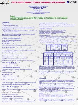
1. Table 1 - Values of ||Px*||, ||Px*d||, and ||Px* Px*d|| for all 3 combinations. ||Px*|| ||Px*d|| ||Px* Px*d|| 1 48.82892.518248.8817 2 0.02521.08861.0886 3 0.25601.08861.0886 Table 2 - Values of the matrices Px* and Px*dfor the 3 combinations. Combination 1 Combination 2 Combination3 Px* Px*d Px* Px*d Px* Px*d Abstract An important issue in control structure selection is plant ”stabilization”. The paper presents a way to select measurement combinations c as controlled variables, such that when c is controlled at a constant setpoint, the effects of disturbances on the states are minimized. • 1. Introduction • Regulatory control layer: • main objective: ”stabilize” the plant • ”Stabilization”: Includes both modes which are mathematically unstable (modes with RHP poles) as well as ”drifting” modes which need to be kept within limits to avoid operational problems. • By avoiding “drift” (keeping all states close to their nominal values we are able to avoid problems resulting from nonlinear effects. • Goal: Select secondary controlled variables (c=y2) such that we minimize the effect of disturbances (d) on the weighted states (y1=Wx). • 2. Previous work: Perfect Indirect Control • Consider that we have the following linear model: • In summary, the main result in this paper can be summarized as follows: • Theorem:LetPxddenote the steady-state transfer function fromdtoxwithc=Hykept constant. Then ||Pxd||2is minimized by selectingH=GxTĞ1Ğy†, , where † indicates the pseudo-inverse. • 4. Application to Distillation • Distillation column: 82 states (41 compositions and 41 liquid holdups). • Manipulated variables:reflux flow rate (L) and vapor boilup (V) • Disturbances: feed flow rate (F) and fraction of liquid in the feed (qF) • Measurements: flow rates (L, V, D, and B). • Combinations of states used: • Combination 1: Bottom and top compositions are the primary variables. Most common choice. • Combination 2: W was selected as being the transpose of Gx (W=GxT). • Combination 3: Wwas calculated solving min||[PxPxd]||2. • For each combination, matrix H was determined using Eq. 5. The resulting values of the 2-norm of ||Px||, ||Pxd||, and ||[PxPxd]|| are presented in Table 1. USE OF PERFECT INDIRECT CONTROL TO MINIMIZE STATE DEVIATIONSEduardo Shigueo Hori, Wu Hong KwongFederal University of São Carlos São Carlos/SP – BrazilSigurd SkogestadNorwegian University of Science and TechnologyN-7491 Trondheim - Norway Indirect control: control y1 indirectly by controlling the ”secondary” variables c: where H is the combination of measurements. Making some algebraic manipulations: Pd -effect of disturbances with closed-loop (partial) control of c Pc - effect on y1 of changes inc Ultimate goal: Perfect disturbance rejection: Pd = 0 and Pc = Pc0 Assumptions: 1. #c = #y1 = #u; 2. #y = #u + #d; 3. The matrix Pc0 is invertible. Solution: WhenPc0=I→G=G1 and Gd=Gd1. 3. Extension: Minimum State Deviation In this case #y1 > #u, so Pd=0is not possible. Instead we want to minimize the norm of Pxd. Consider the following linear model: Although the choice of top and bottom compositions as primary variables (combination 1) is able to control perfectly these two variables (the closed-loop gains relating the disturbances to the bottom and top compositions are zero), the gains of the states in the middle of the column are very large (above 0.7) (see Table 2). This choice doesn’t give good rejection of the implementation error (see matrix Px in Table 2). As expected (session 3), the results presented in Table 1 confirm that the use of W=GxT is an optimum choice. The effect of disturbance in the states is: • 5. Conclusions • 1. It is possible to control perfectly (having perfect disturbance rejection and minimizing the implementation error effects) any combination of the states if we have enough measurements available. • 2. It is shown the importance of the use of the combination of states as primary variables. • 3. Although the choice of the top and bottom compositions of a distillation column is good to reject perfectly the disturbances, it fails in the rejection of the implementation error and also it doesn’t give a good control of the states in the middle of the column. • 4. The choice of W=GxT proved to be the best choice if the objective is to keep the states as close as possible to their desired (nominal) values. • 5. It rejects very well both disturbances and implementation errors, although it doesn’t give perfect control of the top and bottom compositions. • References • Skogestad, S, 2004, Control structure design for complete chemical plants. Comp. Chem. Eng. 28, 219. • Skogestad, S., and I. Postlethwaite, 1996, Multivariable Feedback Control. John Wiley & Sons, London. • Strang, G, 1980, Linear Algebra and its Applications. Academic Press, New York. • Acknowledgments • The financial support of The National Council for Scientific and Technological Development (CNPq/Brasil) and Coordenação de Aperfeiçoamento de Pessoal de Nível Superior (CAPES/Brasil) is gratefully acknowledged. Px and Pxd represent the effect of the disturbances and implementation errors in the states Define the primary variables as linear combinations of the states (y1=Wx): What is the optimal choice of W that minimizes the value of Pxd in Eq. 8? Assuming W=GxT: • Gx(GxTGx)-1GxT is called projection matrix. • The product Gx(GxTGx)-1GxTGxdis the closest point to Gxd. • Thus, the choice W=GxTgives the minimum value ofPxd • W=GxTis optimum for any choice ofPc0non-singular, i.e., result is not restricted to Pc0=I. • W can be arbitrarily chosen by the designer according to the objective of the process.