Stability Analysis for Control Systems
Stability Analysis for Control Systems. Compiled By: Waqar Ahmed Assistant Professor Mechanical UET, Taxila. Sources for this Presentation 1. Control Systems, Western Engineering, University of Western Ontario, Control, Instrumentation & electrical Systems

Stability Analysis for Control Systems
E N D
Presentation Transcript
Stability Analysis for Control Systems Compiled By: Waqar Ahmed Assistant Professor Mechanical UET, Taxila Sources for this Presentation • 1. Control Systems, Western Engineering, University • of Western Ontario, Control, Instrumentation & • electrical Systems • 2. ROWAN UNIVERSITY, College of Engineering, Prof. John Colton
Characteristic Equation of a System Characteristic Equation
Roots of Characteristics Equations • Its very simple to find out roots of a characteristic equation • Replace ‘s’ with a factor jω Characteristic Equation • Substituting the s symbol we get Characteristic Equation • Now solving this equation we get the roots • The roots will have 2 parts, one imaginary and one real • Real part is denoted with σ-axis and imaginary part with jw-axis, as shown on next slide
Real and Imaginary Axis for Roots of a Characteristic Equation Now lets discuss why and how can we say, right hand side of this graph is unstable region and left hand side is stable? What is inverse Laplace Transform of 1/(s-1)? What is inverse Laplace Transform of 1/(s+1)? Answer to above 2 questions will answer the query
Relation between Roots of Characteristic Equation and Stability
A Question Here • Is it really possible and feasible for us to calculate roots of every kind of higher order characteristic equation? • Definitely no! • What is the solution then? • Routh-Herwitz Criterion
Routh-Hurwitz Criterion • The Hurwitz criterion can be used to indicate that a characteristic polynomial with negative or missing coefficients is unstable. • The Routh-Hurwitz Criterion is called a necessary and sufficient test of stability because a polynomial that satisfies the criterion is guaranteed to be stable. The criterion can also tell us how many poles are in the right-half plane or on the imaginary axis.
Routh-Hurwitz Criterion • The Routh-Hurwitz Criterion: The number of roots of the characteristic polynomial that are in the right-half plane is equal to the number of sign changes in the first column of the Routh Array. • If there are no sign changes, the system is stable.
Solution: Since all the coefficients of the closed-loop characteristic equation s3 + 10s2 + 31s + 1030 are positive and exist, the system passes the Hurwitz test. So we must construct the Routh array in order to test the stability further.
Solution (Contd) • It is clear that column 1 of the Routh array is • it has two sign changes (from 1 to -72 and from -72 to 103). Hence the system is unstable with two poles in the right-half plane.
Example of Epsilon Technique: Consider the control system with closed-loop transfer function:
Considering just the sign changes in column 1: • If is chosen positive there are two sign changes. If is chosen negativethere are also two sign changes. Hence the system has two poles in the right-half plane and it doesn't matter whether we chose to approach zero from the positive or the negative side.
Steady State Error: Test Waveform for evaluating steady-state error
Steady-state error analysis Unity feedback H(s)=1 R(s) C(s) E(s) + G(s) - System error E(s) C(s) R(s) Non-unity feedback H(s)≠1 + G(s) - H(s) Actuating error
Steady-state error analysis Consider Unity Feedback System (1) (2) Substitute (2) into (1) (3)
Steady-state error • Final value theorem • Step-input: R(s) = 1/s • 2. Ramp-input: R(s) = 1/s2 3. Parabolic-input: R(s) = 1/s3
Exercise • Determine the steady-state error for the following inputs for the system shown below: • Step-input r(t) = u(t) • Ramp-input r(t) = tu(t) • Parabolic-input r(t) = t2u(t)