Download
1 / 75
910 likes | 1.58k Vues
A Discussion of CPU vs. GPU. CUDA Real “Hardware”. CPU vs. GPU Theoretic Peak Performance. *Graph from the NVIDIA CUDA Programmers Guide, http://nvidia.com/cuda. CUDA Memory Model. CUDA Programming Model. Memory Model Comparison. OpenCL CUDA . CUDA vs OpenCL.

E N D
CPU vs. GPUTheoretic Peak Performance *Graph from the NVIDIA CUDA Programmers Guide, http://nvidia.com/cuda
Memory Model Comparison OpenCL CUDA
A Control-structure Splitting Optimization for GPGPU Jakob Siegel, Xiaoming Li Electrical and Computer Engineering Department University of Delaware
CUDA Hardware and Programming Model • Grid of Thread Blocks • Blocks mapped to StreamingMultiprocessors (SM) SIMT • Manages threads in warps of 32 • Maps threads to Streaming Processors (SP) • Threads start together but are free to branch *Graph from the NVIDIA CUDA Programmers Guide, http://nvidia.com/cuda
Host Device Kernel 1 Kernel 2 Grid 1 Block (0, 0) Block (0, 1) Block (1, 0) Block (1, 1) Block (2, 0) Block (2, 1) Grid 2 Block (1, 1) Thread (0, 2) Thread (0, 1) Thread (0, 0) Thread (1, 1) Thread (1, 0) Thread (1, 2) Thread (2, 1) Thread (2, 2) Thread (2, 0) Thread (3, 1) Thread (3, 2) Thread (3, 0) Thread (4, 1) Thread (4, 2) Thread (4, 0) Thread Batching: Grids and Blocks • A kernel is executed as a grid of thread blocks • All threads share data memory space • Athread blockis a batch of threads that can cooperatewith each other by: • Synchronizing their execution • For hazard-free shared memory accesses • Efficiently sharing data through a low latency shared memory • Two threads from two different blocks cannot cooperate *Graph from the NVIDIA CUDA Programmers Guide, http://nvidia.com/cuda
What to Optimize? • Occupancy? • Most say that the maximal occupancy is the goal. • What is occupancy? • Number of threads that actively run in a single cycle. • In SIMT, things change. • Examine a simple code segment • If (…) • … • Else • …
SIMT and Branches(like SIMD) • If all threads ofa warp execute the same branchthere is no negative effect. Instruction unit SP SP SP SP if { } time
SIMT and Branches • But if only one thread executesthe other branchevery thread hasto step though allthe instructions ofboth branches. Instruction unit SP SP SP SP if { } else { } time
Occupancy • Ratio of active warps per multiprocessor to the possible maximum.Effected by : • shared memory usage(16KB/MP*) • registers usage(8192reg/MP*) • block size(512 t/b*) * For a NVIDIA G80 GPU compute model v1.1
Occupancy and Branches • What if the register pressure of the two equally computational intense branches differ? If-branch: 5 registers Kernel: 5 registers else-branch: 7 registers This adds up to a maximum simultaneous usage of 12 registers Limits Occupancy to 67% for a block size of 256 t/b
Branch-Splitting: Example branchedkernel() { ifcondition load data for if branch perform calculations else load data for else branch perform calculations end if } if-kernel() { ifcondition load all input data perform calculations end if } else-kernel() { if !condition load all input data perform calculations end if }
Branch-Splitting • Idea: Splitting the kernel into two kernels • Each new kernel contains a branch of the original kernel • Adds overhead for: • additional kernel invocation • additional memory operations • Still all threads have to execute both branches But: One Kernel runs with 100% occupancy
Synthetic Benchmark: Branch-Splitting branchedkernel() { load decision mask load data used by all branches if decision mask[tid] == 0 load data for if branch perform calculations else // mask == 1 load data for else branch perform calculations end if } if-kernel() { load decision mask if decision mask[tid] == 0 load all input data perform calculations end if } else-kernel() { load decision mask if decision mask[tid] == 1 load all input data perform calculations end if }
Synthetic Benchmark: Linear Growth Decision Mask • Decision Mask: Binary mask that defines for each data element which branch to take.
Synthetic Benchmark:Linear Growing Mask • Branched version runs with 67% occupancy • Split version:If-kernel 100%Else-kernel 67% else branch executions
Synthetic Benchmark: Random Filled Decision Mask • Decision Mask: Binary mask that defines for each data element which branch to take.
Synthetic Benchmark:Random Mask • Branch execution according toa randomly filled decision mask • Worst case single kernel version = Best case for the split version • Every thread steps through the Instructions of both branches 15% else branch executions
Synthetic Benchmark:Random Mask Branched version:every thread executes both branches and the kernel runs at 67% occupancy Split version:every thread executes both kernels but one kernel runs at100% occupancy the other one at 67% else branch executions
Benchmark: Lattice Boltzmann Method (LBM) • The LBM models Boltzmann particle dynamics on a 2D or 3D lattice. • A microscopically inspired method designed to solve macroscopic fluid dynamics problems.
LBM Kernels (I) • loop_boundary_kernel(){ • load geometry • load input data • if geometry[tid] == solid boundary • for(each particle on the boundary) • work on the boundary rows • work on the boundary columns • store result • }
LBM Kernels (II) • branch_velocities_densities_kernel(){ • load geometry • load input data • if particles • load temporal data • for(each particle) • if geometry[tid] == solid boundary • load temporal data • work on boundary • store result • else • load temporal data • work on fluid • store result • }
Splited LBM Kernels • if_velocities_densities_kernel(){ • load geometry • load input data • if particles • load temporal data • for(each particle) • if geometry[tid] == boundary • load temporal data • work on boundary • store result • } • else_velocities_densities_kernel(){ • load geometry • load input data • if particles • load temporal data • for(each particle) • if geometry[tid] == fluid • load temporal data • work on fluid • store result • }
Conclusion • Branches are generally a performance bottleneck in any SIMT architecture • Branch Splitting might seem and probably is counter productive on most architectures other than a GPU • Experiments show that in many cases the gain in occupancy can increase the performance • For a LBM implementation we reduced the execution time by more than 60% by applying Branch Splitting
Software-based predication for AMD GPUs Ryan Taylor Xiaoming Li University of Delaware
Introduction • Current AMD GPU: • SIMD (Compute) Engines: • Thread processors per SIMD engine • RV770 and RV870 => 16 TPs/SIMD engine • 5-wide VLIW processor (compute cores) • Threads run in Wavefronts • Multiple threads per Wavefront depending on architecture • RV770 and RV870 => 64 Threads/Wavefront • Threads organized into quads per thread processor • Two Wavefront slots/SIMD engine (odd and even)
AMD GPU Arch. Overview Hardware Overview Thread Organization
Motivation • Wavefront Divergence • If threads in a Wavefront diverge then the execution time for each path is serialized • Can cause performance degradation • Increase ALU Packing • AMD GPU ISA doesn’t allow for instruction packing across control flow operations • Reduce Control Flow • Reduce the number of control flow clauses to reduce clause switching
Motivation This example uses hardware predication to decide whether or not to execute a particular path, notice there is no packing across the two code paths. if (cf == 0) { t0 = a + b; t1 = t0 + a; t2 = t1 + t0; e= t2 + t1; } else { t0 = a - b; t1 = t0 - a; t2 = t1 – t0; e= t2 – t1; } 01 ALU_PUSH_BEFORE: ADDR(32) CNT(2) 3 x: SETE_INT R1.x, R1.x, 0.0f 4 x: PREDNE_INT ____, R1.x, 0.0f UPDATE_PRED 02 ALU_ELSE_AFTER: ADDR(34) CNT(66) 5 y: ADD T0.y, R2.x, R0.x 6 x: ADD T0.x, R2.x, PV5.y ..... 03 ALU_POP_AFTER: ADDR(100) CNT(66) 71 y: ADD T0.y, R2.x, -R0.x 72 x: ADD T0.x, -R2.x, PV71.y ...
Transformation if (cond) ALU_OPs1; output = ALU_OPs1; else ALU_OPs2; output = ALU_OPs2; if (cond) pred1 = 1; else pred2 = 1; ALU_OPS1; ALU_OPS2; output = ALU_OPS1 *pred1+ALU_OPS2*pred2; Before Transformation After Transformation This example shows the basic idea of the software-based predication technique.
Approach – Synthetic Benchmark if (cf == 0) { t0 = a + b; t1 = t0 + a; t0 = t1 + t0; e= t0 + t1; } else { t0 = a - b; t1 = t0 - a; t0 = t1 – t0; e= t0 – t1; } t0 = a + b; t1 = t0 + a; t0 = t1 + t0; end = t0+ t1; t0 = a - b; t1 = t0 - a; t0 = t1 – t0; if (cf == 0) pred1 = 1.0f; else pred2 = 1.0f; e = (t0-t1)*pred2 + end*pred1; Before Transformation After Transformation
Approach – Synthetic Benchmark Reduction in Clauses from 3 to 1 01 ALU_PUSH_BEFORE: ADDR(32) CNT(2) 3 x: SETE_INT R1.x, R1.x, 0.0f 4 x: PREDNE_INT ____, R1.x, 0.0f UPDATE_PRED 02 ALU_ELSE_AFTER: ADDR(34) CNT(66) 5 y: ADD T0.y, R2.x, R0.x 6 x: ADD T0.x, R2.x, PV5.y 7 w: ADD T0.w, T0.y, PV6.x 8 z: ADD T0.z, T0.x, PV7.w 03 ALU_POP_AFTER: ADDR(100) CNT(66) 9 y: ADD T0.y, R2.x, -R0.x 10 x: ADD T0.x, -R2.x, PV71.y 11 w: ADD T0.w, -T0.y, PV72.x 12 z: ADD T0.z, -T0.x, PV73.w 13 y: ADD T0.y, -T0.w, PV74.z 01 ALU: ADDR(32) CNT(121) 3 y: ADD T0.y, R2.x, -R1.x z: SETE_INT ____, R0.x, 0.0f VEC_201 w: ADD T0.w, R2.x, R1.x t: MOV R3.y, 0.0f 4 x: ADD T0.x, -R2.x, PV3.y y: CNDE_INT R1.y, PV3.z, (0x3F800000, 1.0f).x, 0.0f z: ADD T0.z, R2.x, PV3.w w: CNDE_INT R1.w, PV3.z, 0.0f, (0x3F800000, 1.0f).x 5 y: ADD T0.y, T0.w, PV4.z w: ADD T0.w, -T0.y, PV4.x 6 x: ADD T0.x, T0.z, PV5.y z: ADD T0.z, -T0.x, PV5.w 7 y: ADD T0.y, -T0.w, PV6.z w: ADD T0.w, T0.y, PV6.x Two 20% Packed Instructions One 40% Packed Instruction
Results – Synthetic Benchmarks A reduction in ALU instructions improves performance in ALU bound kernels. Control flow reduction improves performance by reducing clause switching latency.
Results – Synthetic Benchmark Percent improvement in run time for varying packing ratios for 4870/5870
Results – Lattice Boltzmann Method Percent improvement when applying transformation to one path conditionals.
Results – Other (Preliminary) • N-queen Solver OpenCL (applied to one kernel) • ALU Packing => 35.2% to 52% • Runtime => 74.3s to 47.2s • Control Flow Clauses => 22 to 9 • Stream SDK OpenCL Samples • DwtHaar1D • ALU Packing => 42.6% to 52.44% • Eigenvalue • Avg Global Writes => 6 to 2 • Bitonic Sort • Avg Global Writes => 4 to 2
Conclusion • Software based predication for AMD GPU • Increases ALU packing • Decreases Control Flow • Clause switching • Low overhead • Few extra registers needed if any • Few additional ALU operations needed • Cheap on GPU • Possibility to pack them in with other ALU operations • Possible reduction in memory operations • Combine writes/reads across paths • AMD recently introduced this technique in their OpenCL Programming Guide with Stream SDK 2.1
A Micro-benchmark Suite for AMD GPUs Ryan Taylor Xiaoming Li