Download
1 / 90
970 likes | 1.53k Vues
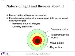
Nature of light and theories about it. Fourier optics falls under wave optics Provides a description of propagation of light waves based on two principles Harmonic (Fourier) analysis Linearity of systems. Quantum optics. Electromagnetic optics. Wave optics. Ray optics. Topics.

E N D
Nature of light and theories about it Fourier optics falls under wave optics Provides a description of propagation of light waves based on two principles Harmonic (Fourier) analysis Linearity of systems Quantum optics Electromagnetic optics Wave optics Ray optics
Topics Week 1: Review of one-dimensional Fourier analysis Week 2: Two-dimensional Fourier analysis Weeks 3-4: Scalar diffraction theory Weeks 5-6: Fresnel and Fraunhofer diffraction Week 7: Transfer functions and wave-optics analysis of coherent optical systems Weeks 8-9: Frequency analysis of optical imaging systems Week 10: Wavefront modulation Week 11: Analog optical information processing Weeks 12-13: Holography
Week 1: Review of One-Dimensional Fourier Analysis Descriptions: time domain and frequency domain Principle of Fourier analysis Periodic: series Sin, cosine, exponential forms Non-periodic: Fourier integral Random Convolution Discrete Fourier transform and Fast Fourier Transform A deeper look: Fourier transforms and functional analysis
Basic idea: what you learned in undergraduate courses A periodic function f(t) can be expressed as a sum of sines and cosines Sum may be finite or infinite, depending on f(t) Object is usually to determine Frequencies of sine, cosine functions Amplitudes of sine, cosine functions Error in approximating with finite number of functions Function f(t) must satisfy Dirichlet conditions Result is that periodic function in time domain, e.g., square wave, can be completely characterized by information in frequency domain, i.e., by frequencies and amplitudes of sine, cosine functions
Historical reason for use of Fourier series to approximate functions Breaks periodic function f(t) into component frequencies Response of linear systems to most periodic waves can be analyzed by finding the response to each ‘harmonic’ and superimposing the results)
Basic idea: what you learned in undergraduate courses (continued) • Periodic means that f(t) = f(t+T) for all t • T is the period • Period related to frequency by T = 1/f0= 2/0 • 0 is called the fundamental frequency • So we have • n0 = 2n/T is nth harmonic of fundamental frequency
How to calculate Fourier coefficients • Calculation of Fourier coefficients hinges on orthogonality of sine, cosine functions • Also,
How to calculate Fourier coefficients (continued) • And we also need
How to calculate Fourier coefficients (continued) • Step 1. integrate both sides: • Therefore
How to calculate Fourier coefficients (continued) Step 2. For each n, multiply original equation by cos nw0t and integrate from 0 to T: 0 0 0 Therefore
How to calculate Fourier coefficients (continued) Step 3. Calculate bn terms similarly, by multiplying original equation by sin nw0t and integrating from 0 to T Get similar result Some rules simplify calculations For even functions f(t) = f(-t), such as cos t, bn terms = 0 For odd functions f(t) = -f(-t), such as sin t, an terms = 0
Calculation of Fourier coefficients: examples Square wave (in class) 1 T T/2 -1
Calculation of Fourier coefficients: examples (continued) Result Gibbs phenomenon: ringing near discontinuity Source: http://mathworld.wolfram.com/FourierSeries.html
Calculation of Fourier coefficients: examples (continued) Triangular wave (in class) +V T T/2 -V
Calculation of Fourier coefficients: examples (continued) Triangle wave result Note that value of terms falls off as inverse square
Other simplifying assumptions: half-wave symmetry Function has half-wave symmetry if second half is negative of first half:
Other simplifying assumptions: half-wave symmetry Can be shown
Conditions for convergence Conditions for convergence of Fourier series to original function f(t) discovered (and named for) Dirichelet Finite number of discontinuities Finite number of extrema Be absolutely convergent: Example of periodic function excluded
Parseval's theorem If some function f(t) is represented by its Fourier expansion on an interval [-l,l], then Useful in calculating power associated with waveform
Effect of truncating infinite series Truncation error function en(t) given by This is difference between original function and truncated series sn(t), truncated after n terms Error criterion usually taken as mean square error of this function over one period Least squares property of Fourier series states that no other series with same number n of terms will have smaller value of En
Effect of truncating infinite series (continued) Problem is that there is no effective way to determine value of n to satisfy any desired E Only practical approach is to keep adding terms until En < E One helpful bit of information concerns fall-off rate of terms Let k = number of derivatives of f(t) required to produce a discontinuity Then where M depends on f(t) but not n
Some DERIVE scripts To generate square wave of amplitude A, period T: squarewave(A,T,x) := A*sign(sin(2*pi*x/T)) For Fourier series of function f with n terms, limits c, d: Fourier(f,x,c,d,n) Example: Fourier(squarewave(2,2,x),x,0,2,5) generates first 5 terms (actually 3 because 2 are zero) To generate triangle wave of amplitude A, period T: int(squarewave(A,T,x),x) Then Fourier transform can be done of this
Exponential form of Fourier Series Previous form Recall that
Exponential form of Fourier Series (continued) Substituting yields Collecting like exponential terms and using fact that 1/j = -j:
Exponential form of Fourier Series (continued) Introducing new coefficients We can rewrite Fourier series as Or more compactly by changing the index
Exponential form of Fourier Series (continued) The coefficients can easily be evaluated
Exponential form of Fourier Series (continued) Sometimes coefficients written in real and complex terms as where
Exponential form of Fourier Series: example Take sawtooth function, f(t) = (A/T)t per period Then Hint: if using Derive, define w = 2p/T, set domain of n as integer
Fourier analysis for nonperiodic functions Basic idea: extend previous method by letting T become infinite Example: recurring pulse v0 t -a/2 a/2 T
Fourier analysis for nonperiodic functions (continued) Start with previous formula: This can be readily evaluated as
Fourier analysis for nonperiodic functions (continued) Using fact that T = 2p/w0, may be written We are interested in what happens as period T gets larger, with pulse width a fixed For graphs, a = 1, V0 = 1
Effect of increasing period T a/T a/T a/T
Transition to Fourier integral We can define f(jnw0) in the following manner Since difference in frequency of terms Dw = w0 in the expansion. Hence
Transition to Fourier integral (continued) Since It follows that As we pass to the limit, Dw -> dw, nDw -> w so we have
Transition to Fourier integral (continued) This is subject to convergence condition Now observe that since We have
Transition to Fourier integral (continued) In the limit as T -> Since f(t) = 0 for t < -a/2 and t > a/2 Thus we have the Fourier transform pair for nonperiodic functions
Example: pulse For pulse of area 1, height a, width 1/a, we have Note that this will have zeros at w = 2anp, n=0,+1, +2 Considering only positive frequencies, and that “most” of the energy is in the first lobe, out to 2ap, we see that product of bandwidth 2ap and pulse width 1/a = 2p
Example of pulse 5 width=1 1 -1/2 1/2 1/10 -1/10 width=0.2
Pulse: limiting cases Let a -> , then f(t) -> spike of infinite height and width 1/a (delta function) -> 0 Transform -> line F(jw)=1 Thus transform of delta function contains all frequencies Let a -> 0, then f(t) -> infinitely long pulse Transform -> spike of height 1, width 0 Now let height remain at 1, width be 1/a Then transform is
Pulse: limiting cases (continued) Now, we are interested in limit as a -> 0 for w -> 0 and w > 0 First, consider case of small w: So when a -> 0, 1/a -> As w moves slightly away from 0, it drops to zero quickly because of w/2a term in denominator (numerator <1 at all times) So we get delta function, d(0)
Properties of delta function Definition Area for any g > 0 Sifting property since
Some common Fourier transform pairs Source: http://mathworld.wolfram.com/FourierTransform.html
Some Fourier transform pairs (graphical illustration) transform function transform function Source: Physical Optics Notebook: Tutorials in Fourier Optics, Reynolds, et. al., SPIE/AIP
Properties of Fourier transforms Simplification: Negative t: Scaling Time: Magnitude:
Properties of Fourier transforms (continued) Shifting: Time convolution: Frequency convolution:
Convolution and transforms A principal application of any transform theory comes from its application to linear systems If system is linear, then its response to a sum of inputs is equal to the sum of its responses to the individual inputs This was original justification for Fourier's work Because a delta function contains all frequencies in its spectrum, if you “hit” something with a delta function, and measure its response, you know how it will respond to any individual frequency The response of something (e.g., a circuit) to a delta function is called its “impulse response” Called “point spread function” in optics Often denoted h(t)
Convolution and transforms (continued) The Fourier transform of the impulse response can be calculated, usually designated H(jw) Therefore if one knows the frequency content of an incoming “signal” u(t), one can calculate the response of the system The response to each individual frequency component of incoming signal can be calculated individually as product of impulse response and that component Total response is obtained by summing all of individual responses That is, response Y(jw) = H(jw)U(jw) Where U(jw) is sum of Fourier transforms of individual components of u(t)
Convolution and transforms (continued) May be visualized as U(jw) H(jw) Y(jw)=H(jw)U(jw) Input Response System